Did you know that over 80% of data-driven decisions in pharmaceuticals, agriculture, and tech rely on comparing multiple groups simultaneously? This is where Analysis of Variance (ANOVA) shines—a method developed by Ronald Fisher in the 1920s to decode patterns hidden within complex datasets. Originally designed for agricultural experiments, it now serves as a backbone for modern research across industries.
At its core, this technique examines whether differences between group averages are statistically significant. It doesn’t just compare two means—like a t-test—but handles three or more, making it indispensable for scenarios like clinical trials or market research. By breaking down variability into systematic and random components, it reveals which factors truly matter.
This article will guide you through its mechanics, from foundational concepts to real-world applications. We’ll explore how it identifies trends in customer behavior, optimizes manufacturing processes, and validates scientific hypotheses. You’ll also learn about its limitations and alternatives for scenarios where simpler tools suffice.
Whether you’re analyzing A/B test results or evaluating policy impacts, understanding this approach empowers sharper decision-making. Let’s uncover how a century-old statistical tool remains vital in today’s data-rich world.
Key Takeaways
- ANOVA compares three or more group means efficiently, reducing error rates in multi-group studies.
- Developed by Ronald Fisher, it originated in agriculture but now drives innovation in tech and healthcare.
- The method separates data variability into explainable and random components for clearer insights.
- Common applications include clinical trials, quality control, and behavioral research.
- While powerful, it requires normally distributed data and equal variances between groups.
- Modern software has made ANOVA accessible to non-statisticians without sacrificing rigor.
Introduction to ANOVA in Statistical Analysis
What if you could compare three or more strategies in a single experiment—while minimizing errors? This capability defines the power of the anova test, a cornerstone technique for researchers and data teams. Unlike simpler comparisons, it handles complex scenarios where multiple groups require simultaneous evaluation.
Overview of ANOVA in Research
Imagine testing three diabetes medications. Each drug represents a group, and blood sugar levels are the measured outcome. Here, the one independent variable (medication type) influences results. This method identifies whether any drug performs significantly better—without inflating error risks from repeated t-tests.
Key advantages include:
- Streamlined comparison of multiple groups in controlled experiments
- Clear separation of systematic effects from random variability
- Scalability for studies with one independent variable across diverse fields
Purpose and Relevance in Data Science
In marketing, teams might analyze sales performance across four regions. The independent variable (geography) helps pinpoint top-performing areas. Data scientists use these insights for feature selection—prioritizing variables that drive meaningful differences.
Consider a tech firm optimizing app load times. By testing variations across user demographics, they validate hypotheses about performance bottlenecks. This approach turns raw data into actionable strategies, bridging theoretical models with real-world impact.
Whether refining clinical protocols or A/B testing campaigns, this method transforms ambiguity into clarity. It’s not just about numbers—it’s about making smarter decisions with confidence.
Defining Core Components in Group Comparisons
Imagine a clinical trial testing three blood pressure medications. Researchers measure diastolic readings—the dependent variable—while controlling dosage amounts as the independent variable. This scenario illustrates why precise terminology matters when evaluating multiple groups.

Key Definitions and Concepts
The method compares group means—average values like crop yields across fertilizer types. For instance:
- Independent variable: Fertilizer brands (controlled factor)
- Dependent variable: Corn production per acre (measured outcome)
Valid results require three assumptions:
| Assumption | Description | Example |
|---|---|---|
| Normality | Data follows bell-shaped distribution | Blood pressure readings in 1,000 adults |
| Homogeneity | Equal variances across groups | Test scores from classrooms with similar sizes |
| Independence | Observations aren’t influenced by others | Separate patient groups in drug trials |
The null hypothesis states all means are equal—like assuming three teaching methods yield identical exam averages. Tests calculate whether observed differences exceed random chance.
In agriculture, this approach might compare wheat yields across four irrigation systems. Each system represents a level of the water management factor. By verifying assumptions, researchers ensure conclusions about optimal methods remain trustworthy.
Types and Variations of ANOVA Methods
Imagine optimizing a mobile app’s user interface across five different layouts. To determine which design performs best, researchers need tools that handle multi-group comparisons. This is where selecting the right type of ANOVA becomes critical.
One-Way ANOVA: Single-Factor Insights
The one-way ANOVA evaluates one independent variable across multiple levels. For example, testing three drug dosages (low, medium, high) on patient recovery times. It answers whether dosage levels significantly affect outcomes—ideal for controlled experiments with a single focus.
Two-Way and Full Factorial Designs
When studying interactions between two independent variables, like marketing campaigns (email, social media) and regions (urban, rural), two-way ANOVA shines. It reveals how variables combine—do urban customers respond better to emails? This method uncovers hidden synergies or conflicts in complex datasets.
| Method | Use Case | Variables | Strength |
|---|---|---|---|
| One-Way | Drug efficacy trials | 1 independent | Simplifies single-factor analysis |
| Two-Way | Consumer behavior studies | 2 independent | Identifies interaction effects |
| Welch’s | Unequal group variances | Robust adjustment | Works with non-homogeneous data |
| Ranked | Ordinal data (e.g., survey scores) | Non-parametric | Bypasses normality assumptions |
Specialized Approaches for Unique Scenarios
Welch’s ANOVA adjusts for unequal variances between groups—useful when comparing manufacturing batches from different factories. Ranked ANOVA handles ordinal data like customer satisfaction tiers. These methods expand applications to real-world data that rarely meets textbook assumptions.
Choosing the right type depends on experimental design and data characteristics. A/B testing might use one-way, while product development teams often leverage two-way for multi-factor optimization. Each method offers a lens to transform raw numbers into strategic insights.
Core Terminology and Assumptions in ANOVA
Clear definitions form the backbone of reliable statistical testing. Misinterpreting terms like dependent variable or factor can lead to flawed conclusions—a risk professionals can’t afford when comparing multiple groups.
Dependent and Independent Variables
The independent variable is the controlled factor—like fertilizer types in crop studies. Researchers manipulate it to observe effects on the dependent variable, such as plant growth. Consider these contrasts:
| Variable Type | Role | Example |
|---|---|---|
| Independent | Controlled input | Marketing channels (email, social) |
| Dependent | Measured outcome | Sales conversion rates |
In drug trials, dosage (independent) influences recovery time (dependent). Precise definitions ensure experiments test what they intend.
Factors, Levels, and Hypotheses
A factor represents an independent variable with multiple levels. Testing three teaching methods? The factor is “instruction style,” with each method as a level. This structure clarifies comparisons between groups.
The null hypothesis claims no difference exists between group means. For example:
- Null: All ad campaigns produce equal website traffic
- Alternative: At least one campaign outperforms others
Valid results depend on three assumptions—normality, equal variances, and independence. Violating these undermines conclusions, making pre-test checks essential. Tools like ANOVA methodology provide frameworks to verify these conditions systematically.
By mastering these terms, analysts transform raw data into trustworthy insights—whether optimizing supply chains or evaluating educational programs.
Interpreting the ANOVA Test: F Statistic and Outcomes
How do researchers determine if a new drug outperforms existing treatments—or if regional sales differences matter? The answer lies in decoding two critical metrics: the F ratio and p-values. These tools transform raw data into actionable conclusions, separating meaningful patterns from random noise.

Calculating the F Ratio
The F ratio measures whether group differences exceed natural variability. It compares:
- Between-group variance: Differences caused by experimental factors
- Within-group variance: Natural fluctuations in data
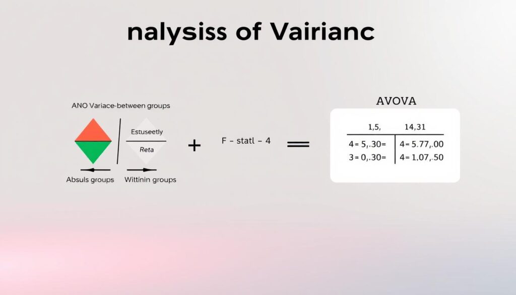
Formula: F = (Between-group variance) / (Within-group variance). Higher values suggest stronger evidence against the null hypothesis. In a clinical trial testing pain relievers, an F ratio of 4.8 would indicate treatment effects outweigh random patient responses.
| Variance Type | Calculation | Role | Example |
|---|---|---|---|
| Between-Group | Differences in group averages | Measures treatment impact | Drug A vs. B vs. C results |
| Within-Group | Spread within each group | Captures natural error | Patient variations in same drug group |
Understanding P-values and Statistical Significance
A p-value quantifies the probability of observing results if no real difference exists. Most studies use a 0.05 threshold:
- p statistically significant
- p ≥ 0.05: Differences could be random
Marketing teams might find a p-value of 0.03 when comparing ad campaigns. This suggests a 3% chance the observed sales boost occurred randomly—strong evidence to adopt the winning strategy.
Even small outcome differences matter. In manufacturing, a 2% defect reduction across three factories could yield an F ratio justifying process changes. By analyzing both metrics, we turn uncertainty into confident decisions.
Application Examples and Use in Research
Pharmaceutical breakthroughs and marketing campaigns share a secret weapon: structured group comparisons. This approach transforms raw observations into validated strategies, whether testing life-saving drugs or optimizing ad spend.
Clinical Trials and Experimental Design
Consider a diabetes study comparing three medications. Researchers measure blood sugar levels (dependent variable) across patient groups receiving different drugs (independent variable). ANOVA determines if any treatment outperforms others—without conducting separate t-tests that inflate error risks.
Key steps include:
- Defining dosage as the controlled factor
- Tracking hemoglobin A1C changes over 12 weeks
- Testing the hypothesis that all drugs have equal effects
Business and Marketing Analytics
A retail chain tests four regional sales strategies. Marketing channels (independent variable) are analyzed against revenue growth (dependent variable). The method reveals whether social media campaigns outperform email blasts in specific demographics.
| Strategy | Region | Sales Lift |
|---|---|---|
| Influencer partnerships | Northeast | 18% |
| Email campaigns | Midwest | 9% |
| Local radio ads | South | 14% |
Tech firms use similar approaches to compare user engagement across app versions. By isolating variables like load time or interface design, teams pinpoint what truly drives conversions. These methods turn complex data into clear roadmaps for innovation.
Limitations and Considerations in Using ANOVA
What separates robust conclusions from misleading ones in multi-group studies? Even powerful tools require careful handling—especially when dealing with real-world data that rarely fits textbook conditions. Let’s examine critical constraints professionals face when applying this method.
Data Distribution and Outlier Impact
The method assumes normally distributed data with equal variances. Skewed distributions or extreme values distort group means, inflating error rates. For example:
- A single outlier in clinical trial results can falsely suggest treatment differences
- Unequal variances between two groups may violate homogeneity assumptions
Consider manufacturing quality checks: if one batch contains defective items (outliers), comparing average defect counts becomes unreliable. Pre-test checks like Shapiro-Wilk normality tests help verify assumptions before analysis.
When to Consider Alternative Methods
While effective for comparing multiple variables, this approach can’t identify specific group differences. Post-hoc tests like Tukey’s HSD become essential for pairwise comparisons. Key scenarios demanding alternatives include:
| Situation | Challenge | Alternative |
|---|---|---|
| Small samples | Low power to detect effects | Non-parametric Kruskal-Wallis |
| Unequal variances | Inflated Type I errors | Welch’s t-test for two groups |
| Ordinal data | Violates normality | Mann-Whitney U test |
Marketing teams analyzing regional sales might use ANOVA initially—but switch to robust tests if data shows heavy skewness. Always verify assumptions through residual plots and Levene’s test before trusting results.
Conclusion
How do data-driven teams confidently navigate complex group comparisons? By leveraging a method that balances rigor with practicality. This approach—central to modern research—helps professionals separate meaningful patterns from random noise, whether testing medications or optimizing marketing campaigns.
We’ve explored how comparing group means requires clear definitions: independent variables like fertilizer types, dependent outcomes like crop yields, and hypotheses that guide inquiry. From one-way designs assessing single factors to factorial models decoding interactions, each variation addresses unique experimental needs.
Real-world applications prove its versatility. Clinical trials rely on it to validate drug efficacy, while businesses use it to compare regional sales strategies. Yet even powerful tools have boundaries. Assumptions like normality and equal variances demand verification—missteps here risk flawed conclusions.
For those analyzing multi-group data, remember: this method shines when questions focus on differences rather than specifics. Pair it with post-hoc tests for granular insights. As industries evolve, mastering these principles remains vital for turning raw data into decisions that shape outcomes.
Ready to deepen your expertise? Explore advanced techniques like mixed-effects models or Bayesian adaptations. Every dataset tells a story—equip yourself to read it with clarity and confidence.
FAQ
What distinguishes one-way ANOVA from two-way ANOVA?
A one-way ANOVA evaluates differences between group means when there’s one independent variable (e.g., comparing sales across three regions). A two-way ANOVA examines how two independent variables (e.g., marketing strategy and season) interact to affect a dependent variable, revealing both main effects and interactions.
When should researchers avoid using ANOVA?
If data violates key assumptions—like non-normal distribution, unequal variances, or outliers—ANOVA may produce misleading results. Alternatives like Welch’s ANOVA or non-parametric tests (e.g., Kruskal-Wallis) are better suited for skewed data or small sample sizes.
How do you interpret the F-statistic in ANOVA results?
The F-statistic compares variance between groups to variance within groups. A higher value suggests greater differences among group means. Researchers compare it to a critical value from F-tables or use the p-value to determine statistical significance (typically p
Can ANOVA handle categorical and continuous variables?
Yes. ANOVA uses categorical independent variables (e.g., product type) to test their effect on a continuous dependent variable (e.g., customer satisfaction scores). However, it requires the dependent variable to be normally distributed within each group.
What real-world applications benefit from ANOVA testing?
In clinical trials, it might compare drug efficacy across dosage levels. Businesses use it to assess how pricing tiers impact sales. For example, a two-way ANOVA could analyze how ad campaigns (variable 1) and store locations (variable 2) jointly influence revenue.
Why is the null hypothesis critical in ANOVA?
The null hypothesis assumes no difference between group means. Rejecting it (via a significant p-value) implies at least one group differs. Post-hoc tests like Tukey’s HSD then identify which specific pairs of groups drive the variance.
How does factorial ANOVA expand on basic methods?
Factorial ANOVA evaluates multiple independent variables and their interactions. For instance, a 3×2 design might test how three training methods and two experience levels affect employee productivity, revealing if certain methods work better for specific experience groups.


