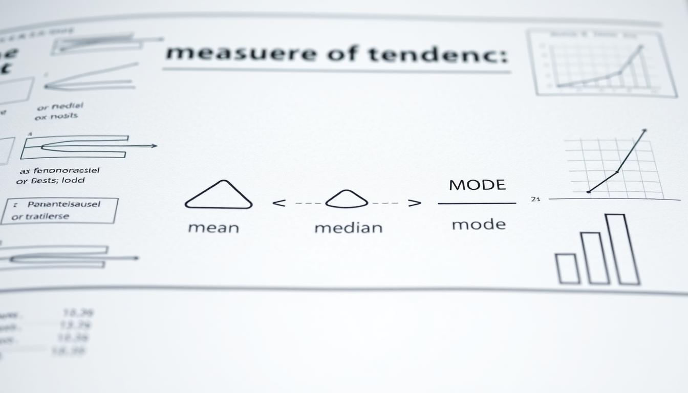
Did you know 85% of data-driven decisions rely on three core metrics to simplify complex information? Whether analyzing sales trends or public health patterns, professionals depend on central tendency measures to identify the “heart” of their datasets. These tools cut through noise, revealing what truly matters in a sea of numbers.
At its core, this approach helps answer critical questions: What’s the typical value? Where does most data cluster? By mastering mean, median, and mode, innovators transform raw figures into strategic insights. The arithmetic mean – often called the average – remains foundational, though its siblings offer unique advantages in skewed distributions.
This guide demystifies these concepts through real-world scenarios, from pricing strategies to performance analytics. We’ll explore how tech leaders use these principles to optimize operations and why researchers consider them indispensable. By the end, you’ll wield these tools with confidence, ready to uncover hidden patterns in your own projects.
Key Takeaways
- Central tendency metrics identify typical values in datasets, simplifying complex information
- Mean, median, and mode each serve distinct purposes depending on data distribution
- The arithmetic mean remains crucial despite sensitivity to extreme values
- Proper application enhances decision-making across industries
- Real-world examples bridge theory and practical implementation
- Mastery empowers professionals to communicate data insights effectively
Introduction to Statistical Analysis & Central Tendency
Every meaningful insight begins with numbers that tell a story. Consider a retail chain tracking daily sales: without organized figures, managers couldn’t spot trends or allocate resources effectively. This process of transforming raw numbers into actionable knowledge lies at the core of data examination.
Understanding the Role of Data in Analysis
Accurate information forms the backbone of informed decisions. A marketing team analyzing customer ages, for instance, might collect responses from 1,000 surveys. Clean, well-structured data sets allow professionals to identify patterns – like whether most buyers fall into the 25-34 age bracket.
Errors in collection distort results. Imagine calculating average delivery times without accounting for regional holidays. Such oversights lead to flawed strategies. Reliable samples ensure findings reflect reality, whether studying voter preferences or product satisfaction rates.
Why Central Tendency Is Essential
Three primary tools simplify complex datasets. The mean calculates an equal balance point, while the median finds the middle value – crucial when extreme figures skew results. Mode reveals the most frequent occurrence, useful for categorical data like preferred payment methods.
Take income analysis in a small town: if nine residents earn $50k yearly and one earns $2 million, the mean distorts reality. Here, the median better represents typical earnings. This principle helps urban planners allocate resources fairly or assists HR teams in setting competitive salaries.
By mastering these concepts, analysts cut through noise to uncover what truly matters. They transform spreadsheets into strategies, proving that numbers – when understood – speak volumes.
Overview of Measures of Central Tendency
What do household incomes, baseball batting averages, and e-commerce sales figures have in common? They all demand precise summarization to reveal their true story. Three fundamental tools achieve this by pinpointing a dataset’s gravitational center.
Defining Mean, Median, and Mode
The arithmetic mean balances all numbers equally. Add every value in your data set and divide by the count. While effective for symmetrical distributions, one extreme value can shift this average significantly – like a billionaire moving a neighborhood’s income mean.
The median resists such distortions by marking the middle position. Arrange values from smallest to largest; the central number wins. This makes it ideal for skewed data, such as housing prices where luxury homes exist alongside modest ones.
Mode identifies the most frequent occurrence. In a classroom test score set, the mode might reveal 85% scored between 80-89. It shines in categorical data analysis – think product sizes or customer survey responses.
- Mean: Sensitive to all values, best for normal distributions
- Median: Resilient to outliers, perfect for skewed data
- Mode: Reveals popularity peaks in categorical or numerical sets
Consider a tech startup analyzing user session times. The mean could suggest 12 minutes, but if most users stay 3 minutes while a few binge-watch for hours, the median (5 minutes) better represents typical behavior. This distinction helps teams allocate server resources wisely.
Choosing the right tool requires understanding your data’s shape. Symmetrical bell curves favor the mean, while lopsided distributions demand the median. When tracking recurring patterns, mode becomes indispensable. Master these differences, and you’ll transform raw numbers into resonant insights.
Calculating the Mean: Understanding the Arithmetic Average
Retirement planning teams faced a critical question: What age best represents their clients’ workforce exit patterns? The arithmetic mean provided clarity, demonstrating how one calculation can distill years of data into actionable insights.

Step-by-Step Calculation Process
The formula for mean remains elegantly simple:
Mean = (Sum of Values) ÷ (Number of Observations)
Consider five retirement ages: 62, 65, 65, 67, 71.
1. Add all values: 62 + 65 + 65 + 67 + 71 = 330
2. Divide by the count: 330 ÷ 5 = 66
This “balancing act” gives equal weight to every data point. Unlike other methods, the mean doesn’t ignore extremes – a strength and weakness simultaneously.
Implications of Using the Mean
When one executive retires at 85 instead of 71, the mean jumps to 68.8. This 2.8-year shift illustrates its sensitivity to outliers. Yet in symmetrical distributions like test scores, it remains unmatched for accuracy.
Tech analysts prefer the mean for normally distributed metrics like website load times. However, skewed datasets – such as income levels – demand alternative approaches. Master this calculation through practice: Start with grocery receipts or exercise durations to build intuitive understanding.
Tomorrow’s exploration of the median will reveal how to handle distorted data landscapes effectively.
Demystifying the Median in Data Analysis
Urban planners once faced a dilemma: Should they prioritize average income or typical earnings when allocating community resources? This real-world challenge highlights why analysts reach for the median – the true north in skewed data landscapes.
How to Determine the Middle Value
The median divides any set data into two equal halves. Unlike averages swayed by extremes, it pinpoints the exact middle position. Here’s how to calculate it:
- Arrange all values in ascending order
- Identify the central position: (n+1)/2 for odd-numbered sets
- Average two middle values for even-numbered sets
Consider household incomes: $32k, $48k, $55k, $63k, $210k. The median ($55k) better represents typical earnings than the skewed mean ($81.6k). This difference matters when making policy decisions or analyzing real-world economic data.
| Data Set Size | Calculation Method | Example |
|---|---|---|
| Odd (5 values) | 3rd value | 12, 18, 22, 25, 31 |
| Even (6 values) | (3rd + 4th)/2 | 15, 20, 23, 27, 30, 35 → 25 |
Tech teams analyzing app usage times often prefer the median. When most sessions last 2-3 minutes but a few exceed an hour, the median middle value reveals typical user behavior – crucial for optimizing server loads.
Financial analysts use this metric to assess housing prices in mixed neighborhoods. A $5 million mansion won’t distort the median like it would the mean, making comparisons between areas more accurate. Master this technique, and you’ll uncover truths hidden in lopsided datasets.
Applying the Mode in Statistical Analysis
A bustling coffee shop chain faced a critical decision: Should they expand their oat milk inventory or stick with dairy? The mode – the most frequent value in their customer preference survey – revealed 68% chose plant-based options. This simple metric transformed their supply chain strategy overnight.

Advantages for Both Categorical and Numerical Data
The mode shines where other values falter. For categorical data like transportation choices, it identifies the popular pick: 45% of commuters prefer trains in a survey of 1,200 urban workers. In numerical sets, it pinpoints recurring patterns – eight employees clocking exactly 37.5 weekly hours despite varying schedules.
Consider classroom test scores: 72, 85, 85, 85, 90. Here, the mode (85) highlights the most common achievement level, unaffected by one struggling student or high performers. This makes it invaluable when outliers distort average calculations.
However, the approach has limits. A set data with two peaks – like bimodal pizza delivery times (25 minutes and 45 minutes) – requires deeper analysis. No single number tells the full story here. Analysts must then pair the mode with other tools like range or standard deviation.
Tech teams use this metric to optimize app features. When 80% of users click the same menu button daily, designers prioritize its placement. Unlike the median or middle value, the mode directly reflects majority behavior without complex calculations.
Choose this method when working with survey responses, product sizes, or repeated events. But always ask: Does the most frequent value align with our strategic goals? Sometimes, the mode reveals what’s popular – not necessarily what’s optimal.
Measures of Central Tendency, Statistical Analysis: Choosing the Best Metric
What separates insightful data summaries from misleading averages? The answer lies in matching measurement tools to your dataset’s unique characteristics. Three core metrics serve different purposes, with their effectiveness hinging on distribution patterns and extreme values.
Key Selection Criteria
Data type dictates initial choices. The mean works best for numerical sets with normal distributions, while the median protects against skewed results. Categorical data like survey responses demands the mode.
| Scenario | Recommended Metric | Reason |
|---|---|---|
| Normal distribution | Mean | Balances all values equally |
| Skewed income data | Median | Ignores extreme outliers |
| Product size preferences | Mode | Identifies popular choices |
Tech teams analyzing app load times found this distinction crucial. When most requests took 2-3 seconds but 5% exceeded 30 seconds, the median provided realistic performance benchmarks.
Navigating Skewed Landscapes
Urban planners analyzing neighborhood incomes face a common challenge: a few luxury homes distort averages. The $250k mean becomes meaningless when 80% earn under $65k. Here, the median’s middle value tells the true story.
Consider these evaluation steps:
- Plot your data distribution
- Identify outlier concentration
- Test different metrics
- Compare results against business goals
E-commerce platforms use this approach daily. When most orders total $45 but holiday shoppers spend $500+, the median prevents overstocking premium items. The right choice transforms numbers into narratives that drive smart decisions.
Impact of Data Distribution and Outliers on Central Tendency
Data patterns reveal truths – unless outliers distort the picture. Skewed distributions pull central tendency metrics away from reality, making metric selection critical. A symmetrical bell curve lets the mean shine, while lopsided data demands the median’s resilience.
Analyzing Skewed Distributions
Positive skewness occurs when most values cluster left with a long right tail – think income data where most earn under $100k, but CEOs pull the mean upward. Negative skew flips this pattern, like retirement ages where early departures dominate. The arithmetic mean becomes unreliable here, while the median anchors to the majority.
Consider app load times: 90% under 3 seconds, but 10% at 15+ seconds. The mean (4.2s) misleads developers, while the median (2.8s) reflects user experience. This divergence impacts server allocation and customer satisfaction metrics.
Strategies for Managing Outliers
Detect extremes using:
- Interquartile range (IQR) fences
- Z-scores beyond ±3
- Visual tools like box plots
Tech teams often trim outliers – removing the top/bottom 5% of response times. Alternatively, transformations like logarithms normalize skewed data. For income studies, reporting both mean and median creates transparency.
Urban planners analyzing housing prices use this dual approach. A $2M mansion won’t shift the median neighborhood value, preserving affordability insights. By pairing metrics with distribution awareness, analysts turn distorted data into decisive action.
Conclusion
Data-driven professionals know that the right metric acts as a compass in numerical chaos. The mean balances all values equally but falters with skewed data. The median resists outliers, anchoring insights to typical experiences. The mode highlights recurring patterns – whether popular product sizes or customer preferences.
Choosing between these tools requires understanding your data set. Symmetrical distributions favor the mean’s precision. Skewed landscapes demand the median’s stability. Categorical analysis thrives with mode’s focus on frequency. Urban planners and tech teams alike transform raw numbers into strategic clarity through this discernment.
Outliers remain critical considerations. A single extreme value can distort averages while leaving medians untouched. Analysts combat this through visual distribution checks and IQR calculations – techniques that separate meaningful trends from statistical noise.
Master these tools, and you’ll communicate insights with newfound authority. Explore real-world applications: optimize pricing strategies using mode, assess housing markets via median, or refine user experiences with mean calculations. Let this guide serve as your trusted mentor in navigating data’s complexities.
Ready to elevate your analytical rigor? Revisit key concepts through practical examples, and discover how blending innovation with methodological discipline drives smarter decisions. The journey from spreadsheets to strategies begins here.
FAQ
How does skewness affect mean and median differently?
In skewed distributions, the mean shifts toward the tail due to extreme values, while the median remains closer to the majority of data. For example, in income data with high earners, the mean overestimates “typical” earnings, making the median a more reliable metric.
When should mode be prioritized over mean or median?
Mode excels with categorical data (e.g., survey responses like “favorite color”) or numerical datasets with repeating values. It identifies the most frequent category or value, offering clarity in scenarios where averages or midpoints aren’t meaningful.
What’s the fastest way to calculate the median for large datasets?
Sort data in ascending order first. For odd-numbered sets, the middle value is the median. For even numbers, average the two central values. Tools like Excel or Python’s Pandas library automate this process efficiently.
Why is the mean sensitive to outliers?
The arithmetic mean includes every value in its calculation. Extreme values disproportionately influence the sum, pulling the average away from the central cluster. For instance, a single
FAQ
How does skewness affect mean and median differently?
In skewed distributions, the mean shifts toward the tail due to extreme values, while the median remains closer to the majority of data. For example, in income data with high earners, the mean overestimates “typical” earnings, making the median a more reliable metric.
When should mode be prioritized over mean or median?
Mode excels with categorical data (e.g., survey responses like “favorite color”) or numerical datasets with repeating values. It identifies the most frequent category or value, offering clarity in scenarios where averages or midpoints aren’t meaningful.
What’s the fastest way to calculate the median for large datasets?
Sort data in ascending order first. For odd-numbered sets, the middle value is the median. For even numbers, average the two central values. Tools like Excel or Python’s Pandas library automate this process efficiently.
Why is the mean sensitive to outliers?
The arithmetic mean includes every value in its calculation. Extreme values disproportionately influence the sum, pulling the average away from the central cluster. For instance, a single $1M salary in a small company inflates the mean salary unrealistically.
Can a dataset have multiple modes?
Yes. Bimodal (two modes) or multimodal distributions occur when multiple values share the highest frequency. For example, exam scores clustering at 75 and 90 suggest two groups of performance, which the mean or median might obscure.
How do outliers impact central tendency metrics?
Outliers skew the mean significantly but leave the median mostly unaffected. Analysts often use the interquartile range (IQR) to detect and manage outliers, ensuring metrics reflect the dataset’s core trends accurately.
What makes the median ideal for ordinal data?
Ordinal data (e.g., rankings like “low, medium, high”) lacks consistent intervals. The median identifies the middle rank without assuming equal distances between categories, preserving the data’s inherent structure better than the mean.
M salary in a small company inflates the mean salary unrealistically.
Can a dataset have multiple modes?
Yes. Bimodal (two modes) or multimodal distributions occur when multiple values share the highest frequency. For example, exam scores clustering at 75 and 90 suggest two groups of performance, which the mean or median might obscure.
How do outliers impact central tendency metrics?
Outliers skew the mean significantly but leave the median mostly unaffected. Analysts often use the interquartile range (IQR) to detect and manage outliers, ensuring metrics reflect the dataset’s core trends accurately.
What makes the median ideal for ordinal data?
Ordinal data (e.g., rankings like “low, medium, high”) lacks consistent intervals. The median identifies the middle rank without assuming equal distances between categories, preserving the data’s inherent structure better than the mean.


