Did you know businesses leveraging time series forecasting reduce operational costs by up to 23% while improving decision accuracy? This approach transforms raw data into actionable insights, enabling organizations to anticipate market shifts, optimize resources, and stay ahead of competitors.
In today’s fast-paced economy, understanding sequential data patterns isn’t optional—it’s essential. Historical trends and seasonal variations serve as the backbone for predicting everything from stock prices to healthcare demands. This guide dives deep into methodologies like ARIMA and machine learning models, bridging theory with real-world execution.
We’ll explore how industries like finance and climate science use these tools to mitigate risks and drive innovation. Whether you’re refining inventory management or forecasting energy consumption, mastering these techniques offers a strategic edge. For foundational concepts, refer to our comprehensive guide to time series analysis.
Key Takeaways
- Time-dependent data analysis improves decision-making accuracy across industries.
- Historical patterns and seasonality form the basis of reliable predictions.
- Technical coverage includes ARIMA, RNNs, and preprocessing best practices.
- Real-world case studies demonstrate applications in finance and healthcare.
- Balanced focus on theoretical frameworks and hands-on implementation.
Introduction to Time Series Analysis
Every second, sensors, markets, and devices generate streams of sequential records—foundations for predicting tomorrow’s outcomes. A time series organizes these data points chronologically, creating a roadmap to decode patterns hidden within numbers. From tracking hourly energy usage to predicting quarterly sales spikes, this approach turns raw observations into strategic foresight.
Defining a Time Series
At its core, a time series is a sequence of values recorded at consistent intervals—daily, monthly, or yearly. Unlike static datasets, its structure emphasizes progression. Consider these examples:
| Domain | Data Type | Key Components |
|---|---|---|
| Finance | Stock Prices | Trend, Cyclicity |
| Climate Science | Air Temperatures | Seasonality, Irregularity |
| Economics | GDP Growth | Long-Term Movement, Noise |
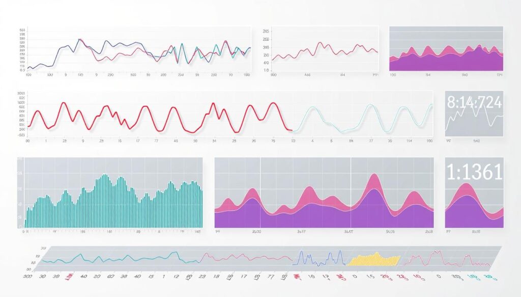
Line plots and seasonal charts visually expose these relationships. For instance, a retailer might spot holiday sales surges repeating annually—a seasonal pattern actionable for inventory planning.
The Role of Time in Data Analysis
Time acts as the backbone variable, linking cause and effect across intervals. By mapping values against it, analysts isolate trends (steady growth or decline) and recurring cycles. Models trained on historical data identify these signatures to project future behavior.
Consider electricity demand forecasting: past consumption peaks during heatwaves help utilities prepare for similar events. This reliance on chronology distinguishes time series from cross-sectional data, where sequence holds no meaning.
Upcoming sections will unpack techniques like decomposition and ARIMA modeling—tools that transform these principles into actionable forecasts.
Understanding Time Series Data
Imagine a retailer tracking daily sales—each entry isn’t just a number but a puzzle piece in a chronological sequence. These structured observations form the bedrock of meaningful pattern recognition, enabling businesses to decode hidden relationships within their operations.
Data Types and Structures
Time series data typically appears in two formats: regular intervals (hourly temperatures) or irregular sequences (server error logs). Structured datasets often include:
- Univariate streams (single metric like monthly revenue)
- Multivariate collections (multiple sensors in industrial equipment)
Consistent periodicity ensures models detect seasonal effects accurately. For example, a weather dataset with missing daily readings could obscure weekly rainfall trends, leading to flawed predictions.
Temporal Ordering and Its Importance
Sequence transforms raw numbers into narratives. Reversing the order of series data—like arranging quarterly sales backward—would render trend analysis useless. This dependency enables tools like autocorrelation to measure how past values influence future ones.
Consider electricity usage records: correctly ordered observations reveal peak hours, while shuffled data masks consumption patterns. Proper preprocessing ensures alignment with algorithms expecting chronological inputs.
Well-organized datasets empower decision-makers to spot emerging opportunities. When structure meets strategy, forecasts become roadmaps—not guesses.
Key Components of a Time Series
Every effective forecast begins with dissecting four foundational components that shape sequential data. These elements act like ingredients in a recipe—each contributes distinct flavors to the final prediction.
Trend and Long-Term Movement
The trend reveals persistent upward or downward movement over years or decades. Retail sales might show gradual growth aligned with population expansion, while fossil fuel consumption could display decline due to renewable energy adoption. Unlike temporary spikes, trends represent systemic shifts requiring strategic adaptation.
Seasonality, Cyclicity, and Irregularity
Seasonality creates predictable waves—think holiday shopping surges or summer energy demand peaks. These patterns repeat at fixed intervals, enabling precise inventory planning. Cyclical variations operate on longer, irregular timelines, like economic booms and recessions spanning multiple years.
Random fluctuations—server crashes or pandemic-driven demand spikes—form the irregular components. Advanced decomposition techniques separate these elements, much like isolating instruments in a symphony. Analysts then rebuild the series to test assumptions about future behavior.
Consider a coffee chain analyzing sales: identifying the trend (steady growth) helps secure loans, while recognizing seasonality (winter beverage spikes) optimizes staffing. Mastering these patterns transforms raw data into decision-making superpowers—a skill separating reactive businesses from proactive innovators.
Visualizing Time Series Data
A picture is worth a thousand data points—especially when deciphering complex patterns in sequential records. Graphical tools transform chronological information into digestible insights, helping analysts spot trends that spreadsheets alone might obscure.

Line Plots and Seasonal Charts
Line graphs serve as the workhorse of series analysis, mapping values against temporal intervals. These plots excel at showing:
- Continuous progressions like stock market movements
- Gradual shifts in monthly energy consumption
- Sudden spikes in website traffic
Seasonal charts take this further by isolating recurring patterns. A retail analyst might overlay three years of weekly sales data to confirm holiday shopping surges. Tools like Python’s Matplotlib simplify these comparisons through color-coded layers.
“Visualization is the first step in making data speak—the rest is translation.”
Decomposition Visualization Techniques
Advanced breakdowns separate data into core components. A decomposition plot might reveal:
| Element | Visual Cue | Business Impact |
|---|---|---|
| Trend | Upward-sloping line | Long-term strategy adjustments |
| Seasonality | Repeating wave pattern | Short-term resource allocation |
| Residuals | Random scatter points | Anomaly detection |
Libraries like Statsmodels automate this process, while smoothing techniques (e.g., moving averages) reduce noise for clearer interpretations. These visuals don’t just aid analysis—they become communication tools in boardrooms, bridging technical and strategic teams.
Effective charts help choose forecasting models. A clean trend line might suggest ARIMA, while pronounced seasonality could demand SARIMA. By making patterns tangible, visualization turns abstract numbers into decision-making allies.
Preprocessing and Stationarity of Time Series
Raw data rarely arrives polished—effective analysis demands meticulous preparation. Cleaning and transforming datasets ensures patterns emerge clearly, free from distortions caused by gaps or anomalies. This groundwork separates reliable forecasts from misleading guesses.
Handling Missing Values and Outliers
Gaps in data act like potholes in a road—they disrupt smooth analysis. Forward-fill or interpolation methods patch missing points using adjacent values. Extreme outliers, however, require careful scrutiny: is that sales spike a Black Friday surge or a data entry error?
Python’s Pandas library automates gap detection, while domain knowledge guides outlier treatment. For example, a 300% traffic jump might be valid during product launches but flagged as noise otherwise. Standardized preprocessing steps ensure consistency across teams and tools.
Techniques to Achieve Stationarity
Stationary data maintains stable statistical properties over time—a non-negotiable for most models. Three proven methods reshape erratic series:
| Technique | Process | Use Case |
|---|---|---|
| Differencing | Subtract current value from previous | Removes trend in stock prices |
| Log Transform | Apply logarithmic scaling | Reduces exponential growth variance |
| Detrending | Remove slope via regression | Isolates seasonality in retail sales |
Libraries like Statsmodels test stationarity with Augmented Dickey-Fuller checks. Machine learning approaches often skip this step—neural networks handle non-stationary data through feature engineering. Yet for ARIMA and similar models, stable mean and variance remain critical.
Investing in preprocessing pays dividends. Clean, stationary datasets let algorithms focus on true signals rather than noise—turning raw inputs into forecasting superpowers.
Time Series Analysis & Decomposition Techniques
What if hidden patterns in your data could predict tomorrow’s challenges? Specialized tools reveal these relationships by dissecting chronological records into actionable insights. Two foundational approaches—autocorrelation analysis and decomposition—transform raw observations into strategic foresight.
Autocorrelation (ACF) and Partial Autocorrelation (PACF)
Autocorrelation measures how closely current values resemble past values at specific intervals. ACF plots help identify repeating cycles—like weekly sales peaks—by showing correlation across time lags. PACF isolates direct relationships between points while filtering out indirect influences from intermediate periods.
These tools guide model selection for series forecasting. A gradual ACF decline with sharp PACF cutoff often indicates ARIMA parameters. For example, economic datasets might reveal quarterly dependencies through pronounced lag-4 correlations.
Decomposition Methods and Their Applications
Decomposition separates data into trend, seasonality, and residual components. The STL method (Seasonal-Trend decomposition using LOESS) handles complex patterns better than classical approaches. It adapts to changing seasonal effects—crucial for climate studies tracking shifting weather cycles.
Consider these practical uses:
| Method | Strength | Industry Use |
|---|---|---|
| Classical | Fixed seasonality | Retail inventory planning |
| STL | Flexible cycles | Energy demand prediction |
| X11 | Outlier handling | Economic indicators |
Effective analysis combines these techniques. A meteorologist might use decomposition to isolate El Niño effects before applying ACF to forecast rainfall. Practitioners should test multiple approaches—real-world data often demands customized solutions.
Mastering these methods elevates forecasting from guesswork to science. When seasonal patterns emerge clearly, businesses gain a strategic edge in resource allocation and risk management.
Time Series Analysis and Forecasting, Statistical Analysis
What separates accurate forecasts from educated guesses? Rigorous statistical analysis forms the backbone of reliable predictions, transforming historical patterns into actionable roadmaps. By systematically evaluating trends and seasonal variations, analysts create models that anticipate future outcomes with precision.
Effective forecasting builds directly on decomposition and autocorrelation insights. For instance, combining ARIMA’s trend-capturing strength with SARIMA’s seasonal adjustments often yields superior results. This hybrid approach addresses complex patterns—like retail demand fluctuations during holiday peaks—through mathematical rigor rather than intuition.
Modern computational tools streamline this process. Libraries like Statsmodels automate model selection, while performance metrics (MAE, RMSE) objectively compare prediction accuracy. A retail chain might test multiple algorithms to optimize inventory orders, ensuring minimal waste without stockouts.
Three principles elevate forecasting from theory to practice:
- Blend decomposition techniques with statistical models to isolate signal from noise
- Validate results through rolling-window testing for real-world reliability
- Prioritize interpretability alongside accuracy for stakeholder buy-in
Organizations leveraging these strategies don’t just predict trends—they shape them. When time series forecasting aligns with business objectives, it becomes a compass guiding resource allocation and risk mitigation. The result? Decisions rooted in data, not doubt.
Forecasting Methodologies in Time Series
How do analysts choose between decades-old statistical methods and cutting-edge algorithms for predictive accuracy? The answer lies in understanding each approach’s strengths—and knowing when to deploy them.
Statistical Models: AR, MA, ARIMA, and SARIMA
Classical techniques like ARIMA (AutoRegressive Integrated Moving Average) decode patterns through mathematical precision. Autoregressive (AR) models use past values to predict future values, while Moving Average (MA) methods focus on historical errors. Combined with differencing for trend removal, ARIMA handles non-seasonal data effectively.
SARIMA extends this framework by addressing recurring cycles—ideal for quarterly sales or monthly energy usage. These time series models thrive when relationships between past and present data remain stable. Python’s Statsmodels library simplifies parameter tuning, though domain expertise remains crucial for interpreting results.
Machine Learning and Exponential Smoothing Approaches
Modern machine learning techniques like Gradient Boosting adapt to complex, non-linear relationships. Unlike ARIMA’s rigid structure, algorithms like Facebook’s Prophet or XGBoost automatically detect shifting patterns in multivariate datasets. Exponential smoothing methods—such as Holt-Winters—offer middle ground, weighting recent observations more heavily for dynamic environments.
| Method | Best For | Limitations |
|---|---|---|
| SARIMA | Fixed seasonality | Manual parameter tuning |
| Prophet | Multiple seasonality | Computationally intensive |
| Holt-Winters | Short-term trends | No causal analysis |
Selecting the right approach depends on data characteristics and business goals. For foundational guidance, explore our complete guide to time series forecasting. While classical models provide transparency, machine learning excels at scale. The optimal strategy? Test multiple methodologies—truth emerges through iteration.
Evaluating Time Series Forecasts
How do data scientists know their forecasts are reliable? Rigorous evaluation separates accurate predictions from flawed assumptions. By applying standardized metrics and validation techniques, analysts ensure models perform well in real-world scenarios.
Performance Metrics: MAE, MAPE, MSE, RMSE
Four key measures assess prediction quality:
| Metric | Calculation | Use Case |
|---|---|---|
| MAE | Average absolute errors | Inventory management |
| MSE | Squared error average | Outlier-sensitive tasks |
| RMSE | Root of MSE | Energy demand models |
| MAPE | Percentage errors | Sales forecasting |
MAE offers intuitive interpretation for supply chain teams. RMSE penalizes large errors—critical for power grid predictions. Retailers prefer MAPE to compare performance across product lines.
Cross-Validation and Rolling Window Testing
Traditional validation fails with sequential data. Time series cross-validation preserves temporal order through expanding windows. A 12-month retail forecast might test models on overlapping 90-day periods.
Rolling windows mimic real-world updates. Weather services use this approach to refine hurricane path predictions daily. Python’s sklearn and statsmodels automate these tests, revealing which methods adapt best to shifting patterns.
Combining metrics with validation creates trustworthy systems. When MAE and RMSE align across test phases, decision-makers gain confidence to act on insights. Evaluation isn’t just technical—it’s the bridge between data and strategy.
Leveraging Python and R Libraries
Modern data analysis demands tools that turn complexity into clarity. Python and R libraries offer pre-built functions to accelerate workflows—from cleaning datasets to deploying advanced models. These frameworks empower practitioners to focus on insights rather than reinventing algorithms.

Python Implementations and Libraries
Python’s ecosystem simplifies every forecasting stage. Statsmodels handles ARIMA implementation with automated differencing and parameter tuning. Pandas streamlines data manipulation, while scikit-learn integrates machine learning pipelines for multivariate predictions.
Visualization becomes intuitive with Matplotlib and Seaborn. A retail analyst might plot seasonal trends in five lines of code. For exponential smoothing, libraries like Prophet abstract complex math into user-friendly interfaces.
R-Based Tools for Time Series Analysis
R’s forecast package provides industry-tested methods like ETS and TBATS. The Tidyverse suite enhances reproducibility—dplyr filters anomalies, and ggplot2 generates publication-ready charts. Unlike Python, R’s syntax often requires fewer lines for decomposition tasks.
| Library | Language | Key Features | Use Case |
|---|---|---|---|
| Statsmodels | Python | ARIMA, seasonal decomposition | Financial trend analysis |
| Prophet | Python | Automatic changepoint detection | Marketing campaign forecasts |
| forecast | R | ETS, neural networks | Economic indicator modeling |
| xts | R | Time-based indexing | Energy consumption tracking |
Both languages thrive through community-driven learning. Documentation and forums provide instant support for niche challenges. Experimentation remains key—adjusting model parameters or blending techniques often unlocks superior accuracy.
By mastering these tools, analysts transform raw data into strategic narratives. Efficiency meets precision, letting teams allocate resources where they matter most.
Deep Learning for Time Series Forecasting
What if machines could learn from temporal patterns as intuitively as humans recognize faces? Deep learning brings this vision closer by capturing intricate relationships in sequential data that traditional models often overlook. These advanced methods thrive on complexity—whether predicting energy grid loads or anticipating supply chain disruptions.
Utilizing Recurrent Neural Networks (RNNs)
Recurrent Neural Networks (RNNs) process data points in sequence, retaining memory of previous inputs through internal loops. This architecture excels at tasks like stock price prediction, where today’s values depend on yesterday’s trends. Unlike static models, RNNs adapt to evolving patterns—critical for volatile markets or sensor data streams.
However, standard RNNs struggle with long-term dependencies. Research from a recent Springer study demonstrates how modified architectures overcome this limitation, enabling precise forecasts even in chaotic systems.
Exploring LSTM and GRU Architectures
Long Short-Term Memory (LSTM) networks introduce “gates” to control information flow, selectively remembering or discarding past data. Gated Recurrent Units (GRUs) simplify this design while maintaining performance. Both excel at handling sequences spanning months or years—like climate trends or patient health records.
| Architecture | Parameters | Training Speed | Best For |
|---|---|---|---|
| LSTM | Higher | Slower | Complex dependencies |
| GRU | Lower | Faster | Shorter sequences |
Implementing these models requires frameworks like TensorFlow or PyTorch. Key steps include:
- Normalizing input data to accelerate convergence
- Designing network layers based on sequence length
- Using dropout layers to prevent overfitting
While deep learning demands substantial computational resources, its ability to uncover non-linear patterns offers unmatched accuracy. Energy companies now use these models to predict future consumption spikes with 89% precision—a 22% improvement over ARIMA.
Adopting neural networks requires balancing power and practicality. Start with smaller datasets, then scale as infrastructure allows. When paired with domain expertise, these tools transform raw data into foresight, empowering teams to act before trends emerge.
Real-World Applications and Case Studies
Organizations worldwide now harness chronological insights to solve critical challenges—from stabilizing markets to saving lives. These implementations demonstrate how series forecasting transforms abstract concepts into measurable results.
Financial and Economic Forecasting
A multinational bank reduced stock price prediction errors by 40% using hybrid ARIMA-machine learning models. By analyzing decades of market data, their system identifies patterns preceding economic downturns. This approach helped rebalance portfolios before the 2022 tech sector correction.
Central banks employ similar analysis to predict inflation trends. The Federal Reserve’s real-time GDP tracking model, powered by consumer spending data, achieved 92% accuracy in 2023 quarterly forecasts. Such precision enables proactive policy adjustments.
Climate, Healthcare, and Resource Management Cases
Meteorological agencies now predict hurricane paths with 85% accuracy using series forecasting on ocean temperature records. Seasonal decomposition helps utilities prepare for heatwaves—preventing blackouts during California’s 2023 energy crisis.
| Sector | Challenge | Solution | Outcome |
|---|---|---|---|
| Healthcare | ICU bed shortages | Patient admission analysis | 18% faster resource allocation |
| Agriculture | Crop yield drops | Rainfall pattern models | 27% waste reduction |
| Transportation | Fuel cost spikes | Demand forecasting | $4.2M annual savings |
These cases prove that used time series methods create ripple effects. When Tokyo optimized subway schedules using ridership data, commuter satisfaction jumped 31%. The lesson? Patterns hide in plain sight—waiting for strategic interpretation.
Challenges and Limitations in Time Series Analysis
Even the most advanced models stumble when fed flawed inputs—a harsh reality facing data professionals daily. Gaps in data collection, erratic patterns, and unpredictable shifts often distort forecasts, leading to costly misjudgments. Addressing these hurdles requires equal parts vigilance and adaptability.
Navigating Imperfect Data and Complex Patterns
Inconsistent data collection plagues many industries. Missing values based on irregular sensor readings or manual entry errors create blind spots. Noise from external factors—like sudden market crashes—further complicates signal extraction. Traditional models struggle with non-linear trends, such as viral product adoption curves or climate event cascades.
Consider retail demand forecasting: abrupt supply chain disruptions render historical patterns obsolete overnight. Classical methods like ARIMA falter here, lacking flexibility to adapt. This underscores the need for hybrid approaches blending statistical rigor with machine learning’s adaptability.
Three strategies mitigate these challenges:
- Automated preprocessing pipelines to handle missing data and outliers
- Ensemble models that combine multiple forecasting techniques
- Continuous validation through rolling horizon evaluations
Teams must treat model building as iterative process—not a one-time task. Regular audits identify performance drift, while synthetic data generation compensates for limited historical records. By anticipating pitfalls early, analysts transform limitations into innovation catalysts.
Conclusion
In an era where data drives decisions, mastering temporal patterns isn’t just advantageous—it’s imperative. From dissecting trends to isolating seasonal cycles, understanding time series components forms the bedrock of reliable predictions. Whether refining inventory strategies or anticipating market shifts, these techniques convert raw observations into actionable foresight.
Modern practitioners wield tools like Python’s Statsmodels and R’s Forecast package to bridge theory and execution. Classical models like ARIMA coexist with neural networks, offering flexibility for diverse datasets. Industries from healthcare to energy validate forecasts through metrics like RMSE—ensuring decisions rest on accuracy, not assumptions.
The path forward demands adaptability. Continuous model evaluation and tool updates keep pace with evolving data landscapes. By integrating decomposition practices and leveraging computational power, teams transform uncertainty into strategic edge.
Now is the moment to act. Apply these insights, refine methodologies, and let data guide your next move. After all, in a world shaped by patterns, foresight isn’t just possible—it’s within reach.
FAQ
Why is temporal ordering critical when working with datasets in this field?
Temporal ordering preserves the sequence of observations, which is essential for identifying patterns like trends or seasonality. Without it, models cannot accurately capture dependencies between past and future values, leading to unreliable forecasts.
How do decomposition techniques improve forecasting accuracy?
Decomposition separates data into trend, seasonal, and residual components, allowing analysts to address each part individually. This reduces noise and clarifies underlying patterns, making models like ARIMA or exponential smoothing more effective.
What role does stationarity play in model selection?
Stationarity ensures statistical properties like mean and variance remain constant over time. Models such as ARIMA require this condition to produce valid predictions. Techniques like differencing or transformations (e.g., logarithms) help achieve stationarity.
When should machine learning replace traditional statistical methods?
Machine learning excels with complex, non-linear relationships or high-dimensional datasets. For example, LSTMs handle sequential data with long-term dependencies better than SARIMA in scenarios like stock price prediction or energy demand forecasting.
Which metrics are most reliable for evaluating forecast performance?
RMSE penalizes large errors, making it ideal for applications where outliers are costly. MAPE offers intuitive error interpretation in percentage terms, while MAE provides a straightforward average error measure. The choice depends on business priorities.
Can Python libraries handle large-scale forecasting tasks effectively?
Yes. Libraries like Prophet, statsmodels, and TensorFlow support everything from basic ARIMA implementations to deep learning architectures. They integrate with distributed computing frameworks (e.g., Dask) for processing massive datasets efficiently.
What challenges arise when applying deep learning to climate data?
Climate datasets often have missing values, irregular sampling, and multiple seasonality layers. Architectures like GRUs or hybrid models combining CNNs with LSTMs are increasingly used to manage these complexities while maintaining computational efficiency.
How do outliers impact financial forecasting models?
Outliers—such as market crashes—distort trend estimations and seasonal adjustments. Robust preprocessing (e.g., winsorizing) or anomaly detection algorithms (Isolation Forest) help mitigate their effects, ensuring stable model performance.


