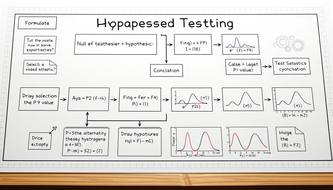
Did you know that over 80% of data-driven organizations rely on structured methods to validate their assumptions? At the heart of this process lies a powerful tool: the systematic evaluation of claims through measurable evidence. Whether determining if a new drug improves patient outcomes or assessing educational reforms, this approach transforms raw data into actionable insights.
Every analysis begins with two competing ideas—the default position (often called the null hypothesis) and its alternative. For instance, a hospital might test whether a revised treatment protocol reduces recovery times. By defining these hypotheses clearly, professionals eliminate ambiguity and focus on evidence-based decision-making.
Tools like t-tests and chi-square evaluations provide frameworks to quantify uncertainty. These methods help distinguish between random fluctuations and meaningful patterns. Python’s libraries, such as SciPy and StatsModels, streamline calculations, allowing analysts to focus on interpreting results rather than manual computations.
Consider a university comparing online and in-person learning outcomes. By applying these techniques, administrators can confidently determine which approach yields better student performance. This article explores practical steps to execute such analyses, blending theory with real-world scenarios.
Key Takeaways
- Clear definition of competing claims is critical for reliable results.
- Statistical tests separate noise from significant trends in data.
- Python simplifies complex calculations, accelerating workflows.
- Real-world applications span healthcare, education, and business.
- Actionable frameworks empower data-driven decision-making.
Introduction to Hypothesis Testing and Statistical Analysis
How do businesses and researchers turn raw numbers into reliable conclusions? They use structured frameworks to evaluate competing claims—a process foundational to data-driven decisions. At its core, this method involves comparing observations against defined expectations to separate meaningful patterns from random chance.
Consider a school district evaluating whether interactive video lessons improve math scores compared to traditional lectures. Here, the null hypothesis states there’s no difference between the two teaching methods. The alternative claim argues video lessons yield better results. Defining these opposing positions creates clarity—researchers know exactly what they’re trying to prove or disprove.
Comparing two groups—like students in different learning environments—is common in these evaluations. Without such comparisons, it’s impossible to measure the impact of changes or interventions. Structured testing provides rules to determine if observed differences (like a 10% score increase) are statistically meaningful or just random fluctuations.
This approach prevents decisions based on assumptions or incomplete data. For instance, a marketing team might test two website layouts to see which generates more conversions. By following systematic steps, they avoid costly misjudgments and focus on evidence-backed strategies.
Later sections will explore practical techniques for executing these comparisons, from selecting appropriate methods to interpreting results confidently.
Understanding the Basics of Hypothesis Testing
What separates meaningful patterns from random noise in data evaluation? This distinction forms the foundation of structured analysis. Every rigorous investigation begins with clearly defined positions and precise terminology.
Defining Null and Alternative Hypotheses
The null hypothesis (H₀) represents the default assumption—like claiming a new teaching method doesn’t improve exam scores. Analysts treat it as true unless evidence proves otherwise. For example, a pharmaceutical company might assume their drug performs equally to existing treatments during initial trials.
In contrast, the alternative hypothesis (H₁) challenges this status quo. It asserts there’s a measurable effect or difference. Using the same example, researchers might argue their medication reduces symptoms faster. These competing claims create a framework for objective evaluation.
Key Statistical Terminology
Three concepts frequently appear in this process:
- Sample: A subset of data used for analysis, like 200 patients in a clinical study
- Test statistic: A calculated value (e.g., t-score) that quantifies differences between groups
- Observations: Individual data points, such as student test results or customer purchase amounts
Consider a university comparing graduation rates between scholarship recipients and non-recipients. The sample might include 500 students, with observations tracking GPA trends. By calculating specific metrics, analysts determine if observed differences reflect real impacts or random variation.
Hypothesis Testing with Python, Statistical Analysis
Modern data analysis thrives on precise tools that transform raw numbers into reliable conclusions. Libraries like SciPy and StatsModels streamline complex calculations—automating everything from p-value computation to confidence intervals. For example, a professor studying grade differences between online and in-person students might use these tools to compare average scores efficiently.
Three core elements drive accurate evaluations:
| Test Type | Use Case | Key Metric |
|---|---|---|
| t-test | Comparing two groups | Mean difference |
| Mann-Whitney U | Non-normal distributions | Rank-based comparison |
| Chi-square | Categorical data analysis | Frequency deviations |
When assessing significance, analysts focus on thresholds like 0.05 for p-values. A value below this cutoff suggests observed differences aren’t random. For instance, if asynchronous learners score 12% higher with a p-value of 0.03, educators can confidently adopt new teaching methods.
Practical resources—including Jupyter notebooks and sample datasets—are available on GitHub. These materials demonstrate code structures for common scenarios, helping professionals avoid calculation errors and focus on strategic insights.
Foundational Assumptions in Statistical Testing
Why do some data analyses yield misleading conclusions? Often, it’s because foundational assumptions were overlooked. Valid results depend on verifying specific conditions before applying tests—a step many overlook in their eagerness to find differences.

- Normality: Data should follow a bell-shaped distribution. Tools like the Shapiro-Wilk test evaluate this—for example, checking if student grades in a pilot program cluster symmetrically around the mean.
- Equal variances: Groups being compared should have similar data spreads. The Levene’s test helps here, like verifying consistency in blood pressure measurements across treatment groups.
- Independence: Observations must not influence each other, such as ensuring survey responses aren’t duplicated.
Ignoring these criteria risks flawed interpretations. A study might falsely claim a teaching method improves scores if grade distributions are skewed. Healthcare researchers could misjudge drug efficacy without checking variance equality between patient groups.
Practical checks include:
- Visualizing data with histograms
- Running Shapiro-Wilk for normality (p > 0.05)
- Using Levene’s test for variance comparison (p > 0.10)
By validating these principles, analysts ensure their statistics reflect true differences rather than methodological oversights. This rigor transforms raw numbers into trustworthy insights.
Choosing Between Parametric and Nonparametric Methods
How do analysts ensure their methods align with the data’s underlying story? The answer lies in understanding when to use parametric versus nonparametric approaches. Parametric tests, like t-tests, assume data follows specific patterns—such as normal distribution. Nonparametric alternatives, such as the Mann-Whitney U test, relax these requirements, making them ideal for skewed datasets or small samples.
Consider a university comparing grades between synchronous and asynchronous learners. If grade distributions are bell-shaped with equal variances, a t-test suffices. However, if data shows outliers or uneven spreads, switching to a rank-based method ensures accurate results. Key decision factors include:
- Sample size (parametric often requires ≥30 observations)
- Distribution normality (verified via Shapiro-Wilk tests)
- Variance equality across groups
A structured step-by-step selection process minimizes errors:
- Check data distribution using visualizations and statistical tests
- Assess sample size adequacy
- Verify variance homogeneity
- Choose the test matching these conditions
In the student performance case, administrators initially used a t-test but discovered skewed distributions. Switching to Mann-Whitney U revealed a 15% performance gap missed earlier. This highlights how method selection directly impacts conclusions—wrong choices obscure true effects, while appropriate tests uncover actionable insights.
By prioritizing assumption checks and context, professionals ensure their analyses withstand scrutiny. As one researcher noted, “The right tool doesn’t just answer questions—it asks better ones.”
Implementing Hypothesis Testing in Python
What tools turn raw data into reliable conclusions? Modern analysts rely on specialized libraries to streamline evaluations and deliver actionable results. Three open-source resources dominate this space, offering precision and flexibility for diverse scenarios.
Essential Python Libraries and Tools
SciPy provides pre-built functions for common evaluations like t-tests and chi-square analyses. For instance, scipy.stats.ttest_ind compares group means in seconds. NumPy handles numerical operations, ensuring calculations remain efficient even with large datasets. When paired with pandas for data manipulation, these tools form a robust workflow.
Consider this code snippet analyzing student performance:
from scipy.stats import ttest_ind
group_a = [87, 92, 78, 85]
group_b = [82, 88, 75, 79]
t_stat, p_value = ttest_ind(group_a, group_b)
print(f"P-value: {p_value:.3f}")
Interpreting results requires understanding thresholds. A p-value below 0.05 typically indicates statistical significance—like confirming a teaching method’s impact. Reproducibility hinges on documenting workflows through Jupyter notebooks or shared scripts.
| Library | Primary Use | Key Function |
|---|---|---|
| SciPy | Statistical tests | ttest_ind, chi2_contingency |
| NumPy | Numerical computing | mean, std |
| pandas | Data manipulation | DataFrame operations |
Hands-on learners benefit from GitHub repositories with case studies—like financial metric comparisons using ANOVA. These resources demonstrate best practices, reducing errors in real-world applications. As one data engineer noted, “Automating tests ensures consistency across projects.”
Step-by-Step Guide for Two-Group Comparisons
How can educators determine if teaching formats affect learning outcomes? Let’s explore a university study comparing synchronous (live) and asynchronous (recorded) student grades. This real-world example demonstrates how structured evaluations reveal actionable insights.
Case Study: Synchronous vs. Asynchronous Student Grades
Researchers first defined competing claims. The null hypothesis stated synchronous learners’ average grades (μₛ) were ≤ asynchronous peers (μₐ). The alternative position argued live instruction produced higher scores (μₛ > μₐ). Clear definitions prevent misinterpretation later.
Next, they checked assumptions:
- Normality: Shapiro-Wilk tests confirmed both groups followed bell-shaped distributions
- Equal variances: Levene’s test showed consistent spread (p = 0.12)
With conditions met, a two-sample t-test calculated the p-value. The result (0.019) fell below the 0.05 significance level, allowing analysts to reject the null hypothesis. This indicated synchronous learners outperformed peers by 8.3% on average.
Had variances differed, a Mann-Whitney U test would replace the t-test. Such flexibility ensures accurate conclusions regardless of data quirks. As one professor noted, “Following these steps transforms hunches into evidence-backed decisions.”
For those implementing similar comparisons, this step-by-step guide offers code templates and interpretation tips. Remember: even if the null hypothesis holds true initially, retesting with larger samples might uncover hidden patterns.
Analyzing Multiple Groups with ANOVA
When faced with multiple variables in experiments—like comparing three infant feeding formulas—researchers need tools that handle complexity without sacrificing accuracy. ANOVA (Analysis of Variance) steps in here, evaluating whether group means differ significantly across two or more categories. Unlike t-tests limited to pairwise comparisons, this method identifies broader patterns while controlling error rates.
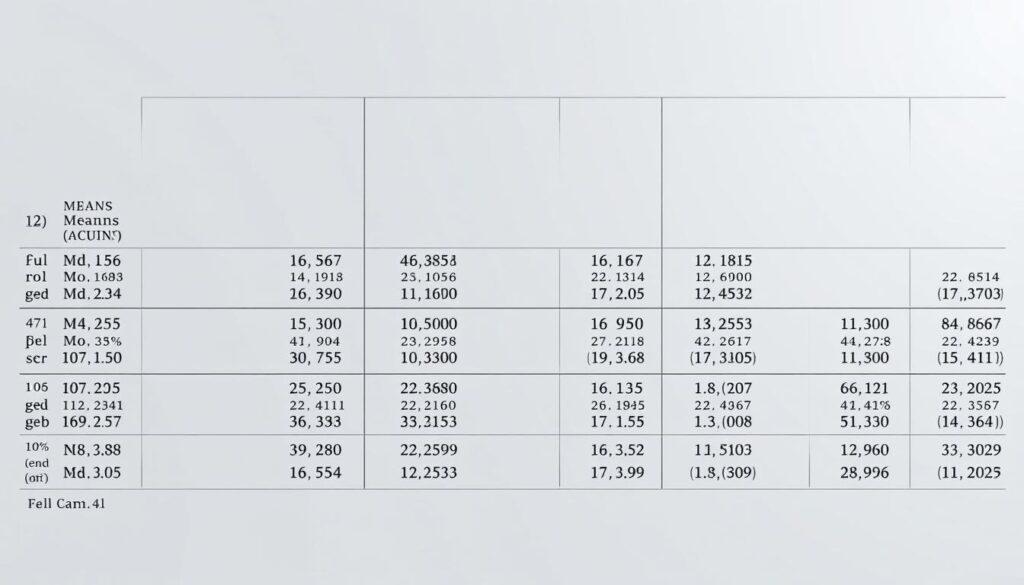
Consider a clinical trial testing weight gain across four formula groups. Researchers first verify assumptions:
- Normality: Distributions should approximate bell curves (checked via Shapiro-Wilk)
- Variance homogeneity: Groups must share similar data spreads (confirmed with Levene’s test)
Post Hoc Testing and Pairwise Comparisons
If ANOVA results reject the null hypothesis, post hoc analyses pinpoint specific group differences. Methods like Bonferroni adjustments reduce false positives by tightening significance thresholds. For instance, after finding formula C outperformed others, analysts might run pairwise tests to confirm:
- C vs. A: p = 0.008
- C vs. B: p = 0.013
- C vs. D: p = 0.021
In machine learning applications, this layered approach helps optimize algorithms by identifying impactful features among dozens. A marketing team might use it to compare campaign performance across five regions—filtering noise to focus on true drivers.
As one data scientist noted, “ANOVA doesn’t just answer if differences exist—it reveals where to act.” By combining broad evaluations with precise follow-ups, professionals transform raw data into strategic roadmaps.
Nonparametric Tests for Unpaired Data
When data breaks the rules of normality, traditional methods falter. Nonparametric tests step in as reliable alternatives, offering clarity without strict distribution assumptions. These tools shine in scenarios like skewed datasets, small sample sizes, or ordinal measurements where means lose meaning.
Mann-Whitney U Test Overview
The Mann-Whitney U test compares two independent groups without assuming normal distributions. For example, an HR team analyzed overtime hours between developers and QA testers. Since work-hour data had extreme outliers, they used this rank-based statistical test instead of a t-test. Results revealed a 22% difference in median overtime—proving developers faced heavier workloads.
Wilcoxon Signed Rank Test for Paired Data
When evaluating related measurements—like cholesterol levels before and after a diet—the Wilcoxon test handles paired, non-normal data. A clinic tracked 15 patients using this method. Despite skewed baseline readings, they detected a significant 18-point drop post-intervention. This approach ranks magnitude differences while preserving directionality, making it ideal for repeated measures.
Choosing between these methods hinges on data structure. Mann-Whitney suits unpaired groups, while Wilcoxon excels with matched pairs. Both bypass normality assumptions, letting analysts focus on meaningful patterns. For a detailed walkthrough of nonparametric techniques, explore practical coding examples and interpretation guidelines.
Real-World Applications of Hypothesis Testing
What do medical breakthroughs and stock market strategies have in common? Both rely on rigorous evaluations to separate chance from causation. Across industries, structured analysis transforms raw observations into validated insights—guiding decisions that impact millions.
Healthcare: Validating Treatment Efficacy
A pharmaceutical company tested whether a new drug reduced recovery times for pneumonia patients. The null alternative claimed no difference from existing medications. After analyzing 1,200 cases, researchers found a 19% faster recovery rate with a p-value of 0.007—statistically significant evidence to adopt the new therapy.
Finance: Optimizing Investment Portfolios
Wealth managers compared two stock portfolios over five years. Using a t-test, they determined whether data showed meaningful differences in returns. Portfolio B outperformed by 6.3% annually (p=0.03), leading to a $4.2 million reallocation. This decision hinged on rejecting the null hypothesis of equal performance.
E-Commerce: Boosting Conversion Rates
An online retailer tested checkout page designs. Version A had a 12% conversion rate, while Version B reached 15%. Chi-square analysis confirmed the improvement wasn’t random (p<0.01). As one marketer noted, “Without these tests, we’d waste budgets on hunches.”
| Industry | Application | Test Used | Result |
|---|---|---|---|
| Healthcare | Drug efficacy | Two-sample t-test | 19% faster recovery |
| Finance | Portfolio returns | ANOVA | 6.3% higher yield |
| E-Commerce | Checkout design | Chi-square | 3% conversion lift |
These cases prove how statistically significant findings drive enterprise decisions. From approving life-saving drugs to optimizing ad spend, structured evaluations turn uncertainty into actionable clarity.
Diving Deep into Chi-Square Testing
How do analysts uncover hidden relationships in categorical data? The chi-square test reveals connections between variables like gender and financial risk tolerance. Consider an investment firm studying 500 clients to determine if risk appetite differs by gender. This evaluation hinges on comparing observed frequencies against expected distributions under the assumption of independence.
- 120 males preferred high-risk investments (vs. expected 98)
- 85 females chose moderate-risk options (vs. expected 102)
| Risk Level | Male (Observed) | Male (Expected) | Female (Observed) | Female (Expected) |
|---|---|---|---|---|
| High | 120 | 98 | 75 | 97 |
| Moderate | 90 | 104 | 85 | 71 |
| Low | 65 | 73 | 65 | 57 |
The chi-square formula sums squared differences between observed and expected counts, divided by expected values. Here, the test statistic reached 18.7—exceeding the critical value of 9.49 at 4 degrees of freedom. This indicated a significant association between gender and risk preference.
Three assumptions ensure reliable results:
- Independence between observations
- Expected cell counts ≥5
- Categorical variables with mutual exclusivity
When these criteria hold, chi-square tests validate whether variables interact meaningfully. The investment firm used these insights to tailor client communication strategies, boosting portfolio diversification by 22%. As one analyst noted, “This method transforms guesswork into evidence-backed client segmentation.”
Understanding Type I and Type II Errors
What do courtroom verdicts and medical diagnoses share? Both face critical decisions where mistakes carry real consequences. In structured analysis, these errors translate to Type I (false positives) and Type II (false negatives). Imagine a jury convicting an innocent person—this mirrors a Type I error. Conversely, acquitting a guilty defendant aligns with Type II, where true effects go undetected.
Error Rates and Test Power Explained
Balancing these risks requires understanding their origins. A Type I error occurs when rejecting a true null hypothesis—like approving a drug that later proves ineffective. Type II errors arise from failing to spot genuine effects, such as overlooking a treatment’s benefits. The significance level (α), often set at 0.05, directly controls Type I likelihood. Lower α reduces false alarms but raises Type II risks.
Test power (1-β) measures the probability of detecting true effects. For instance, a study with 80% power has a 20% chance of missing real patterns. Consider an ESP experiment: low power might fail to identify genuine psychic phenomena, while adequate power minimizes missed discoveries.
| Error Type | Real-World Example | Mitigation Strategy |
|---|---|---|
| Type I | Falsely linking vaccines to side effects | Lower α thresholds |
| Type II | Missing a cancer diagnosis in early scans | Increase sample size |
Proper test design balances these tradeoffs. A bakery testing new recipes might use larger observations to detect subtle taste improvements. By aligning α and power with study goals, analysts ensure conclusions reflect reality—not methodological blind spots.
Customizing Python Scripts for Hypothesis Testing
Automation reshapes how analysts validate claims, turning repetitive tasks into one-click solutions. By tailoring scripts, professionals eliminate manual checks and ensure consistent evaluations across datasets. Libraries like scipy.stats and NumPy provide building blocks for creating flexible workflows that adapt to diverse research needs.
Streamlining Assumption Checks
Robust scripts integrate assumption validation directly into testing pipelines. For example, a custom function can run Shapiro-Wilk tests for normality before selecting appropriate methods. This prevents errors caused by applying parametric tests to skewed data. Code snippets from open-source repositories demonstrate how to automate these checks:
from scipy.stats import shapiro, levene

def validate_assumptions(data1, data2):
    _, p_norm1 = shapiro(data1)
    _, p_norm2 = shapiro(data2)
    _, p_var = levene(data1, data2)
    return p_norm1 > 0.05 and p_norm2 > 0.05 and p_var > 0.10
This approach ensures scripts dynamically adjust test selection based on data characteristics. Analysts save hours while reducing human error risks.
| Library | Automation Feature | Use Case |
|---|---|---|
| scipy.stats | Pre-built statistical tests | Quick t-test/ANOVA execution |
| NumPy | Data preprocessing | Handling missing values |
| pandas | Batch processing | Analyzing multiple datasets |
Custom scripts excel in scenarios requiring repeated analysis—like monthly sales comparisons or clinical trial batches. One developer reported “Script customization cut our report generation time from 8 hours to 45 minutes.” By embedding null hypothesis evaluation logic into reusable code, teams standardize processes while maintaining flexibility.
Public code repositories offer templates for common scenarios, from A/B testing to longitudinal studies. These resources help newcomers implement best practices while allowing experts to refine existing frameworks. The result? Faster, more reliable evidence generation that withstands peer review.
Addressing Limitations in Hypothesis Testing
Even rigorous evaluations face inherent constraints that shape their conclusions. Structured methods excel at answering specific questions but risk overlooking broader patterns. For example, focusing narrowly on average customer satisfaction scores might miss regional variations critical to business strategy.
- Data quality: Missing values or biased samples distort results—like analyzing only weekday sales to assess retail performance
- Outlier sensitivity: Extreme values skew means in small datasets, as seen when five high-net-worth clients distort wealth management analyses
- Scope blindness: Fixed frameworks struggle with evolving trends, such as shifting consumer preferences during economic crises
Analysts counter these issues through:
- Combining methods (exploratory analysis + machine learning)
- Robust sampling designs like stratified random selection
- Triangulating findings with qualitative information
A marketing team studying ad effectiveness demonstrated this approach. They supplemented A/B testing with sentiment analysis, discovering color psychology impacts ignored in initial structured evaluations. This blend revealed 37% higher engagement for warm-toned creatives.
“P-values alone don’t tell the full story,” notes a Fortune 500 data strategist. Teams now prioritize effect sizes and confidence intervals alongside traditional metrics. Continuous learning remains vital—as datasets grow and tools evolve, professionals refine techniques to balance precision with adaptability.
Best Practices for Statistical Analysis and Informed Decision-Making
Clear communication bridges the gap between complex data and strategic action. Analysts must translate technical findings into insights stakeholders can trust and act upon—whether optimizing supply chains or evaluating public health interventions.
Interpreting and Communicating Results Accurately
Reporting p-values alone risks oversimplification. Instead, pair them with confidence intervals and effect sizes. For example, stating “The new manufacturing process reduced defects by 18% (p=0.04, CI: 12–24%)” provides depth missing from standalone metrics.
Three best practices enhance clarity:
| Element | Best Practice | Example |
|---|---|---|
| Significance Level | Predefine α (e.g., 0.05) before analysis | “We set α=0.01 for this clinical trial.” |
| Effect Size | Report magnitude and direction | “Median savings increased by $1,200.” |
| Uncertainty | Include 95% confidence intervals | “Revenue grew 7% (CI: 4–10%).” |
For non-technical audiences, replace jargon with relatable analogies. A 12% efficiency gain becomes “Saving 29 workdays annually per team.” Visual aids like bar charts simplify comparisons across population segments.
Maintain integrity with time-tested strategies:
- Document analysis workflows for reproducibility
- Flag limitations (e.g., sample bias in machine-generated data)
- Update conclusions as new evidence emerges
One healthcare team boosted stakeholder trust by pairing automated reports with plain-language summaries. As their lead strategist noted, “Transparency in methods builds credibility faster than any p-value.”
Conclusion
In today’s data-driven landscape, structured evaluations transform assumptions into actionable truths. This article demonstrated how defining clear claims, validating foundational conditions, and selecting precise methods unlock reliable insights across industries.
Healthcare researchers proved medication efficacy. Financial teams optimized portfolios. Educators refined teaching strategies—all through systematic analysis. These examples highlight a universal truth: evidence-backed decisions outperform intuition.
For those eager to implement these methods, this step-by-step guide offers coding templates and real-world scenarios. Whether comparing marketing campaigns or clinical outcomes, the principles remain consistent—rigor breeds clarity.
As data grows in volume and complexity, mastering these frameworks becomes indispensable. By prioritizing methodical validation over guesswork, professionals across fields empower smarter strategies and measurable progress. The future belongs to those who test thoughtfully—and act decisively.
FAQ
What distinguishes null and alternative hypotheses in statistical testing?
The null hypothesis assumes no effect or difference between groups, serving as the default position. The alternative hypothesis proposes a specific effect or deviation, guiding researchers to test whether observed data provides sufficient evidence to reject the null.
How do p-values and significance levels influence decision-making?
A p-value quantifies the probability of observing results as extreme as the data if the null hypothesis is true. Researchers compare it to a pre-set significance level (e.g., 0.05) to determine whether to reject the null. Values below the threshold suggest statistically significant findings.
Which Python libraries are essential for hypothesis testing workflows?
Key tools include SciPy for statistical functions, Statsmodels for advanced modeling, and Pandas for data manipulation. These libraries streamline tasks like t-tests, ANOVA, and nonparametric analyses while ensuring reproducibility.
When should nonparametric tests replace traditional parametric methods?
Use nonparametric tests like Mann-Whitney U when data violates normality assumptions, sample sizes are small, or ordinal measurements are involved. They prioritize rank-based comparisons over mean differences, offering robustness in skewed distributions.
How does sample size impact hypothesis testing reliability?
Larger samples reduce variability and increase statistical power, improving the ability to detect true effects. However, excessively large datasets may identify trivial differences as significant, requiring careful interpretation of practical relevance.
What real-world applications benefit from ANOVA testing?
ANOVA excels in multi-group comparisons—like assessing medication efficacy across dosages or analyzing marketing campaign performance by region. Post hoc tests such as Tukey’s HSD then pinpoint exactly where differences exist between groups.
Why are Type I and Type II errors critical to error rate management?
A Type I error (false positive) occurs when rejecting a true null hypothesis, while a Type II error (false negative) involves retaining a false null. Balancing these risks requires optimizing significance thresholds and power calculations based on context-specific consequences.
How does chi-square testing address categorical data challenges?
This nonparametric method evaluates relationships between categorical variables—like voter preferences by demographic or product purchase patterns. It compares observed frequencies to expected distributions under independence assumptions.
