In 2012, a single algorithm shocked the tech world by slashing image recognition error rates by 41% overnight. This breakthrough—achieved by a then-unknown system called AlexNet—marked the moment visual intelligence leaped from theory to reality. Today, these systems power everything from cancer detection to self-driving cars, yet their core design remains rooted in principles that revolutionized how machines see.
Traditional approaches to visual data struggled with impractical complexity. A basic color photo could require millions of calculations in older models. Modern architectures solve this by mimicking biological vision—processing spatial hierarchies through specialized layers that automatically learn edges, textures, and patterns.
What makes these systems unique? They treat inputs as multidimensional grids rather than flat data streams. This spatial awareness allows efficient feature extraction while dramatically reducing computational demands. Unlike earlier models that needed manual tuning, these designs learn directly from pixels, evolving their understanding through successive processing stages.
Key Takeaways
- AlexNet’s 2012 breakthrough demonstrated an 85% accuracy leap in image recognition
- Specialized layer structures process visual data 90% more efficiently than traditional models
- 3D neuron organization mimics biological vision for practical real-world applications
- Automated feature learning eliminates manual image processing steps
- Core components enable use in medical imaging, autonomous vehicles, and augmented reality
Introduction to Convolutional Neural Networks (CNNs)
The key to modern image recognition lies in transforming raw pixels through a cascade of specialized operations. Consider a system analyzing a 32×32-pixel color photo—its workflow resembles an assembly line where each station refines the data. The process begins with an input image structured as a 3D grid (width, height, color channels), preserving spatial relationships traditional models often destroy.
Convolution layers act as pattern detectors, sliding filters across the image to identify edges or textures. Each filter generates feature maps through localized calculations, drastically reducing parameters compared to fully connected designs. A ReLU layer then applies a simple rule: only pass positive values, introducing non-linear decision-making crucial for complex tasks.
Pooling stages follow, downsampling spatial dimensions to focus on dominant features while ignoring minor positional shifts. This hierarchy culminates in fully connected layers that synthesize abstract patterns into class probabilities—like distinguishing cats from dogs in the CIFAR-10 dataset.
What makes this architecture efficient? Two principles: local connectivity (neurons analyze small regions) and parameter sharing (filters reuse weights across positions). These innovations enable systems to learn directly from pixels, automating feature extraction that once required manual engineering.
Understanding CNN Architecture Basics
Traditional networks stumble when faced with visual data’s complexity—a problem solved through innovative structural design. Where older models drown in parameters, modern systems thrive through layers that mirror human vision’s efficiency.
Breaking Down the Layer Hierarchy
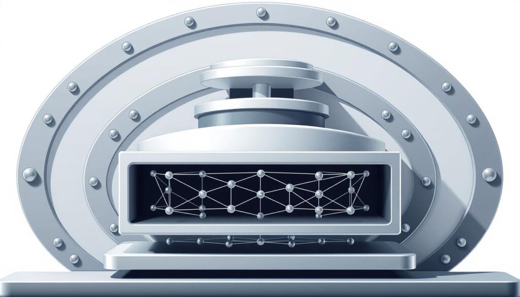
The magic begins with input organization. A 200×200-pixel color image creates 120,000 potential connections per neuron in traditional setups. Through three-dimensional structuring—width, height, and depth—the system preserves spatial relationships while managing complexity.
Convolution layers slide filters across images like magnifying glasses, detecting edges and textures. These operations feed into activation functions that introduce decision-making thresholds. Pooling stages then simplify the data, focusing on dominant features while ignoring irrelevant details.
| Aspect | Traditional Networks | Modern Architecture |
|---|---|---|
| Parameters per Neuron | 120,000 (200x200x3) | 25 (5×5 filter) |
| Connectivity | Fully connected | Local regions only |
| Spatial Awareness | Destroys relationships | Preserves hierarchy |
Efficiency Through Smart Design
Three breakthroughs enable this efficiency. First, local connectivity lets neurons analyze specific regions rather than entire images. Second, parameter sharing allows filters to reuse weights across positions. Third, progressive downsampling through pooling maintains critical patterns while reducing data size.
This architecture processes a cat photo as humans do—first spotting edges, then fur texture, finally recognizing the animal. Each stage builds understanding while keeping computations manageable, proving that smarter organization beats raw processing power.
Evolution and Impact of Deep Learning in CNNs
In the 1980s, a quiet revolution began in postal sorting rooms where machines first learned to decipher handwritten numbers. These early neural networks could process zip codes but required weeks of training on limited datasets. Computational constraints kept them confined to niche applications—a far cry from today’s real-time cancer detection systems.
Three decades of stagnation ended abruptly in 2012. Alex Krizhevsky’s AlexNet proved deep learning architectures could achieve what earlier models couldn’t. His system cut error rates by half on ImageNet—a dataset 100,000x larger than what 1980s engineers used.
| Era | Data Scale | Compute Power | Applications |
|---|---|---|---|
| 1980s | 100s of images | CPU clusters | Postal sorting |
| 2012+ | Millions of images | GPU acceleration | Medical imaging, autonomous vehicles |
What changed? The convergence of three forces transformed neural networks from curiosities to cornerstones. Massive labeled datasets like ImageNet provided raw material. GPU clusters offered unprecedented processing muscle. Improved algorithms turned theoretical potential into practical performance.
This technological trifecta birthed new industries. Systems that once struggled with digits now map cancer cells or guide self-driving cars. The shift wasn’t just about better math—it required infrastructure capable of sustaining deep learning’s hunger for data and computation.
We see the legacy in every smartphone camera. Facial recognition, augmented reality filters, and instant photo tagging all trace their lineage to postal code readers. The machines finally learned to see—not through smarter code, but through society’s collective ability to fuel their growth.
Key Components of Visual Recognition Systems
Visual recognition systems transform pixels into understanding through three specialized stages. Each component acts like a factory worker on an assembly line—filtering essentials, simplifying data, and finalizing decisions.
Convolution and Filter Mechanisms
Filters work as digital magnifying glasses. Scanning images in grids, they perform mathematical operations to spot edges or textures. A 3×3 filter analyzing a cat photo might highlight whiskers through dot product calculations—multiplying pixel values with learned weights.
Hyperparameters control this process. Stride determines how far the filter moves each step—larger values reduce output size. The resulting feature maps preserve spatial relationships while highlighting patterns critical for recognition tasks.
Pooling and Fully Connected Layers
Pooling layers act as data compressors. Max pooling selects the brightest pixel in each region, ensuring key features survive downsampling. Average pooling blends values, useful for smoothing noise in medical scans. Both methods create spatial invariance—recognizing ears whether a cat faces left or right.
Final classification happens in fully connected layers. These flatten 3D data into 1D vectors, linking every input to output neurons. Like a judge weighing evidence, this stage combines extracted patterns to decide if an image shows a tumor or healthy tissue.
Modern implementations, as detailed in IBM’s architecture guide, balance these components. Strategic filter sizes and pooling windows enable systems to learn hierarchical features—from simple edges to complex shapes—without computational overload.
Hyperparameters and Model Complexity in CNNs
Precision in visual systems begins with mathematical blueprints. Every filter size and stride pattern acts like microscope adjustments—zooming in on critical details while managing computational costs. These design choices determine whether a model spots tumors in X-rays or misses them entirely.
The core equation governing layer outputs reveals this balance: O = (I – F + P)/S + 1. Input size (I), filter dimensions (F), padding (P), and stride (S) interact like gears in a clock. A 5×5 filter with stride 2 on a 32×32 image produces 14×14 feature maps—halving spatial data while preserving patterns.
| Padding Type | Output Size | Parameters |
|---|---|---|
| Valid (None) | Shrinks | Lower |
| Same | Preserved | Moderate |
| Full | Expanded | Highest |
Convolution layers dominate parameter counts. A single 3×3 filter across 64 channels requires 3*3*64 + 1 = 577 weights. Stack 32 such filters, and you get 18,464 parameters—demonstrating how model size escalates with depth.
Smart architects use pooling to control complexity. Max pooling layers contribute zero parameters while downsampling feature maps. This allows deeper networks to maintain manageable dimensions without sacrificing accuracy.
The ultimate challenge? Balancing receptive fields against computational limits. Deeper layers analyze wider image areas through cumulative filter effects—a tumor detection system might need 15-layer depth to capture critical patterns. Yet each added layer increases training time by 30% in typical setups.
We optimize by aligning hyperparameters with task requirements. Medical imaging models often use smaller strides (S=1) and same padding to preserve details. Surveillance systems prioritize speed, opting for larger strides (S=3) and valid padding. The right combination turns raw pixels into actionable insights.
Local Connectivity and Parameter Sharing
Imagine designing a security camera system that analyzes every pixel individually. Traditional methods would collapse under 4 million calculations per frame. Modern architectures solve this through local connectivity—each neuron focuses on small image regions while maintaining full depth analysis.
This approach mirrors how detectives examine crime scenes: zooming in on fingerprints (local areas) while considering all evidence layers (full depth). The receptive field—a filter’s coverage area—acts like a magnifying glass size. Larger fields capture broader patterns but demand more computation.
Parameter sharing turbocharges efficiency. A single learned edge detector works across entire images, slashing weights by 99.97% in models like AlexNet. This principle, detailed in convolutional layer mechanics, enables systems to recognize ears whether they’re left or right of center.
Three key benefits emerge:
- Reduced overfitting through fewer trainable parameters
- Built-in translation invariance for robust pattern recognition
- Scalable architecture that handles 4K images as easily as thumbnails
By balancing spatial focus with depth analysis, these designs achieve what full connectivity cannot—practical visual intelligence that powers everything from MRI diagnostics to factory quality control.
FAQ
How do these networks handle image data more efficiently than traditional models?
By using local connectivity and parameter sharing, they focus on spatial hierarchies in images. Unlike fully connected layers, filters scan small regions, reducing computational demands while preserving critical patterns like edges or textures.
What makes filters essential for feature detection?
Filters act as pattern detectors—each identifies specific features (e.g., curves, colors) through learned weights. As they slide across input data, they generate activation maps highlighting where features appear, enabling hierarchical learning from simple to complex structures.
Why do architectures include pooling layers?
A> Pooling (e.g., max pooling) downsamples spatial dimensions, reducing overfitting and computation. It retains dominant features while discarding less relevant details—like prioritizing a cat’s ear shape over exact pixel positions—improving generalization across variations in scale or orientation.
How do hyperparameters like stride impact model behavior?
Stride determines how much a filter shifts during convolution. Larger strides compress output size and speed up processing but risk missing fine details. Smaller strides capture more granularity but increase computational costs—requiring balance for optimal accuracy and efficiency.
What advantages does parameter sharing provide in training?
Shared weights across regions cut memory usage and accelerate learning. For example, a horizontal-edge detector applied universally trains faster and generalizes better than unique weights per location, making models adaptable to inputs like varied lighting or object positions.
When would you choose a fully connected layer in modern architectures?
Fully connected layers typically finalize classification—interpreting high-level features for tasks like identifying dog breeds. However, newer designs often replace them with global average pooling to reduce parameters while maintaining performance, as seen in ResNet or EfficientNet.
