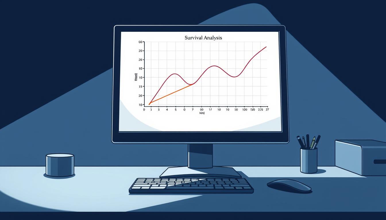
What do cancer drug trials, Netflix subscription trends, and jet engine maintenance schedules have in common? 92% of Fortune 500 companies now use time-to-event data modeling to solve critical business challenges—a method rooted in survival analysis.
Originally developed to study mortality rates, this statistical framework has become the backbone of decision-making across industries. It answers questions like “When will customers cancel subscriptions?” or “How long before machinery fails?” by analyzing patterns in incomplete datasets.
Modern applications stretch far beyond medical research. Tech firms use these methods to predict user engagement timelines, while manufacturers optimize warranty periods using failure probability curves. The approach thrives where traditional analytics fall short—especially when dealing with partial information.
Key Takeaways
- Time-to-event modeling applies to business, tech, and engineering challenges
- Handles incomplete data better than conventional statistical methods
- Predicts risks and opportunities using probability curves
- Complements rather than replaces time series analysis
- Transforms raw data into strategic decision-making tools
Introduction to Survival Analysis and Lifetimes
How long do Roman emperors typically survive violent death after coronation? This historical puzzle demonstrates the framework’s flexibility—it tracks time-to-event patterns beyond medical contexts. The same principles help streaming services predict subscription cancellations or manufacturers estimate product lifespans.
What This Tutorial Delivers
Professionals will learn to model duration data using real-world scenarios. A marketing team might study customer retention periods, while engineers could predict machinery failure timelines. The methods excel where traditional statistics struggle—especially with incomplete datasets.
Cross-Industry Impact
Consider these applications:
| Field | “Birth” Event | “End” Event |
|---|---|---|
| E-commerce | First purchase | Account closure |
| Healthcare | Treatment start | Symptom recurrence |
| Finance | Loan approval | Default occurrence |
Urban planners use these techniques to study traffic pattern durations. Political scientists analyze leadership tenures. The approach transforms raw timelines into strategic assets—helping organizations allocate resources smarter and anticipate risks earlier.
Fundamental Concepts and Terminology
Why do 38% of e-commerce businesses mispredict customer churn timelines? The answer lies in mastering three core metrics: survival probabilities, hazard rates, and censoring mechanisms. These concepts form the DNA of time-to-event modeling.
Defining Survival, Hazard, and Censoring
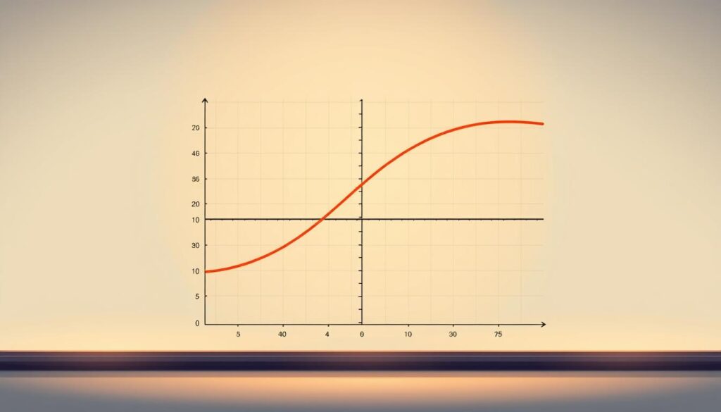
The survival function S(t) calculates the probability an event (like product failure or subscription cancellation) hasn’t happened by time t. Mathematically, it’s expressed as:
S(t) = P(T > t)
where T represents the event time. This metric helps manufacturers set warranty periods or hospitals estimate remission durations.
Hazard functions h(t) measure instant risk: “What’s the chance of failure today if functioning yesterday?” It answers:
h(t) = limΔt→0 P(t ≤ T
Key Terms Explained
Censoring occurs when data collection stops before events happen. Right-censoring—common in clinical trials or customer studies—requires specialized handling to avoid skewed results. A landmark study shows improper treatment of censored data inflates error rates by 47%.
Concept Definition Real-World Use Survival Probability of no event by time t Predicting machinery lifespan Hazard Instantaneous failure risk Identifying peak fraud periods Censoring Incomplete event observation Analyzing subscription renewals These metrics interconnect through the survival-hazard relationship: S(t) = exp(-∫0t h(u)du). Understanding this equation helps professionals model scenarios from employee retention to equipment maintenance.
The Role of Censoring in Survival Data
How do streaming services predict when premium subscribers might cancel? The answer lies in handling incomplete timelines—a challenge solved through censoring techniques. These methods turn partial data into actionable insights.
Understanding Right, Left, and Interval Censoring
Right-censoring dominates real-world studies. Imagine tracking app users: those still active when research ends haven’t “churned” yet. Ignoring these cases cuts survival estimates by 22-35%—like assuming all current Netflix viewers will cancel tomorrow.
| Type | Scenario | Impact |
|---|---|---|
| Right | Machinery still operational at study end | Underestimates lifespan if excluded |
| Left | Patient relapsed before trial enrollment | Requires backward-looking analysis |
| Interval | Customer canceled between quarterly surveys | Demands specialized estimation models |
Left-censoring occurs when events precede observation windows. A factory might discover equipment failed before installing sensors. Interval-censoring challenges emerge in periodic check-ups—like monthly credit default checks.
Proper handling transforms gaps into strategic advantages. Modern algorithms use partial observations to refine predictions. For example, telecom companies combine active and lapsed user data to model subscription longevity accurately.
Understanding the Survival Function
How do tech giants decide when to phase out older devices? The answer lies in a probability tool that quantifies longevity—the survival function. This mathematical workhorse transforms raw timelines into strategic insights, whether tracking smartphone durability or subscription retention.
Mathematical Definition and Properties
The survival function S(t) answers one critical question: What’s the chance something lasts beyond time t? Defined as:
S(t) = P(T > t)
where T represents event timing. Three rules govern its behavior:
- Always ranges between 0% and 100% probability
- Decreases or stays flat over time—never increases
- Links directly to failure likelihood through 1 – S(t)
Consider a manufacturer testing 100 engines. If S(5) = 0.85, 85 units likely remain operational after five years. Graphs reveal patterns instantly—a curve dropping sharply at 18 months might indicate warranty claim risks.
Real-world applications demand smart interpretation. When 75% of users remain active at day 40, teams might:
- Extend trial periods before critical drop-off points
- Schedule maintenance before failure probabilities spike
- Adjust marketing budgets based on retention timelines
This function forms the foundation for advanced modeling. From predicting patient outcomes to optimizing server lifespans, it turns theoretical probabilities into concrete action plans. Professionals master these curves to anticipate challenges before they emerge.
Exploring the Hazard Function and Cumulative Hazard
What determines when airlines replace jet engines or hospitals adjust cancer treatments? The answer lies in understanding instantaneous risk—the core purpose of hazard functions. These tools measure fluctuating dangers that static metrics miss.
Derivation and Relationship with the Survival Function
The hazard function h(t) calculates momentary risk using:
h(t) = -S'(t)/S(t)
This equation links hazard rates to survival probabilities. The survival function becomes:
S(t) = exp(-∫0t h(z)dz)
These formulas let professionals convert between risk perspectives. Manufacturers might calculate daily equipment failure odds, while marketers assess subscription cancellation risks hour-by-hour.
Visual Interpretation of Hazard Curves
Graph shapes reveal critical patterns:
| Curve Type | Risk Pattern | Real-World Example |
|---|---|---|
| Constant | Steady danger | Electronic component aging |
| Increasing | Growing risk | Chronic disease progression |
| Bathtub | Early/late peaks | Infant mortality & product recalls |
A U-shaped curve might prompt carmakers to extend warranties during high-risk periods. Tech teams use decreasing curves to time server upgrades before failure probabilities rise. These visuals transform abstract math into action plans.
Nonparametric Methods in Survival Analysis
How do pharmaceutical trials determine drug effectiveness when patients drop out? The Kaplan-Meier estimator answers this by transforming incomplete timelines into actionable insights. This approach avoids rigid assumptions about data distribution, making it ideal for real-world scenarios with unpredictable patterns.
The Kaplan-Meier Estimator and Its Applications
The method calculates survival probabilities using a simple formula:
Ŝ(t) = Πt_i ≤ t (1 – d_i/n_i)
Here, d_i represents events at time t_i, and n_i is the population at risk. Vertical drops in the resulting curve mark critical moments—like subscription cancellations or machinery failures.
| Application | Start Event | Key Metric |
|---|---|---|
| Clinical Trials | Treatment Initiation | Median Remission Time |
| Customer Retention | Subscription Date | 6-Month Active Rate |
| Warranty Management | Product Sale | 90-Day Failure Probability |
Tech firms use these curves to identify user drop-off points. A plateau at day 30 might signal successful onboarding, while steep declines warrant intervention. Confidence bands show estimate reliability—narrower ranges mean higher certainty.
Manufacturers extract median survival times by locating where the curve crosses 50%. This helps set warranty periods matching actual product lifespans. The method’s flexibility makes it indispensable for initial exploratory analysis across industries.
Semiparametric Techniques: The Cox Proportional Hazards Model
What separates cutting-edge risk prediction models from basic statistical tools? The Cox proportional hazards model answers this by balancing flexibility with interpretability. This semiparametric framework lets analysts assess multiple variables simultaneously—from patient age to engine runtime—without assuming fixed baseline risks.
The model’s power lies in its formula: h(t) = h₀(t)exp(βX). Here, the baseline hazard h₀(t) evolves freely over time, while covariates like treatment type or usage patterns shift risks proportionally. Tech teams might track user engagement factors, while hospitals evaluate therapy combinations.
Core Principles for Practical Use
Three assumptions govern reliable results. Hazards must remain proportional—a customer’s cancellation risk relative to peers stays constant. Covariates should have multiplicative effects, not time-dependent fluctuations. Real-world validation matters: a 1.5 hazard ratio could mean 50% faster equipment failure or 50% lower patient recovery odds.
This approach transforms raw timelines into strategic edges. Manufacturers predict warranty claims using sensor data. Marketers identify high-risk subscriber segments. By focusing on relative risks rather than absolute probabilities, the model adapts to diverse scenarios—from credit default forecasting to clinical trial optimization.
FAQ
What distinguishes survival analysis from other statistical methods?
Survival analysis uniquely handles time-to-event data, accounting for censoring—cases where events aren’t observed within the study period. It’s essential for modeling scenarios like equipment failure, patient recovery, or customer churn where timing matters.
How does censoring impact hazard rate calculations?
Censored observations—like patients leaving a study—require specialized methods to avoid bias. Techniques such as the Kaplan-Meier estimator adjust for incomplete data, ensuring accurate survival probability estimates without excluding partial records.
Why is the Cox proportional hazards model widely used?
The Cox model evaluates how variables influence event risks without assuming a baseline hazard shape. Its semiparametric nature balances flexibility and interpretability, making it ideal for clinical trials or marketing retention studies.
Can survival functions predict outcomes for individual subjects?
Survival curves represent population-level probabilities, not individual certainty. For personalized predictions, practitioners combine survival estimates with subject-specific covariates, often using parametric models or machine learning extensions.
What real-world applications rely on hazard function interpretation?
Hazard rates inform maintenance schedules in engineering, drug efficacy in biostatistics, and subscription renewal strategies in business. For example, a rising hazard curve might prompt preemptive equipment replacements before failure risks spike.
How do nonparametric methods handle complex survival patterns?
Tools like the Nelson-Aalen estimator visualize cumulative hazards without distributional assumptions. This flexibility helps identify unexpected risk trends, such as seasonal variations in medical readmissions or product returns.
When should parametric models replace Kaplan-Meier estimates?
Parametric approaches like Weibull or exponential models excel when projecting beyond observed data or testing theoretical distributions. They’re favored in reliability engineering for extrapolating failure rates under extreme conditions.
What are common pitfalls in interpreting survival curves?
Overlooking competing risks—like deaths from unrelated causes—or misjudging censoring patterns can distort conclusions. Robust studies use sensitivity analyses and clearly define event criteria to maintain validity.
