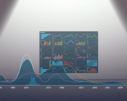
Did you know companies that leverage recurring data patterns achieve 30% higher forecast accuracy than those relying solely on linear projections? These predictable fluctuations—driven by holidays, weather, or cultural rhythms—hold immense strategic value. Recognizing them transforms raw numbers into actionable intelligence.
Seasonality isn’t just about holiday sales spikes or summer tourism booms. It’s the heartbeat of operational planning. Retailers optimize inventory before Black Friday. Farmers align planting cycles with rainfall trends. Energy providers anticipate winter demand surges. Each sector reveals unique rhythms begging to be decoded.
Mastering these patterns requires more than basic observation. Professionals need frameworks to distinguish true cyclicality from random noise. When executed well, this process turns historical data into a crystal ball—predicting opportunities and mitigating risks before competitors react.
Key Takeaways
- Recurring trends impact industries from retail to agriculture
- Accurate pattern recognition boosts forecast precision
- Strategic planning relies on cyclical data interpretation
- Advanced tools separate meaningful trends from anomalies
- Cross-department collaboration maximizes insights
Through real-world examples and practical methodologies, we’ll explore how to transform temporal data into competitive weapons. The journey begins with understanding why these patterns matter—and ends with mastering their application.
Introduction to Seasonal Analysis
Behind every successful forecast lies the untold power of recognizing data rhythms. These repeating waves in information streams help organizations separate predictable cycles from chaotic noise. When harnessed effectively, they become strategic assets driving smarter decisions.
Decoding Cyclical Signals
Pattern detection transforms raw numbers into actionable intelligence. Retailers spot holiday purchase surges six months early. Energy providers predict consumption spikes before winter storms hit. This foresight comes from systematic tracking of recurring peaks and valleys.
Financial institutions use these insights to anticipate market reactions to tax seasons. Agricultural planners align crop rotations with rainfall trends. The latest seasonality detection methods help teams distinguish true cyclicality from random fluctuations.
Effective analysis achieves more than accurate predictions. It exposes anomalies that demand attention—unexpected sales drops during peak periods or unusual energy usage in stable weather. These deviations often signal operational issues or emerging opportunities.
Data-driven organizations leverage these insights to:
- Optimize inventory before demand surges
- Adjust staffing for anticipated busy periods
- Allocate marketing budgets to high-impact windows
Mastering cyclical patterns requires both technical skill and business context. Analysts must interpret data through industry-specific lenses while maintaining statistical rigor. The reward? Turning historical repetitions into future advantages.
Understanding Seasonal Analysis in Time Series
What separates strategic forecasts from guesswork? The answer lies in recognizing predictable repetitions hidden within data streams. These rhythmic fluctuations—whether daily, weekly, or annual—form the backbone of informed decision-making across industries.

Defining Core Concepts
Seasonality manifests as repeating peaks and valleys at fixed intervals. Think ice cream sales tripling every July or utility bills spiking during winter months. Unlike trends showing gradual growth, these patterns reset periodically—like clockwork.
Consider three temporal dimensions:
- Daily: Commuter traffic surges at 8 AM and 5 PM
- Weekly: E-commerce orders double every weekend
- Annual: Hotel bookings peak during holiday seasons
True cyclicality differs from irregular events. Economic recessions create unpredictable dips, while Black Friday sales arrive like calendar alerts. This distinction separates noise from actionable signals.
The Role of Seasonality in Forecasting
Models ignoring recurring patterns risk catastrophic errors. A retailer might stock snowblowers in July or understaff during Christmas rush. One transportation company reduced fuel costs by 18% after aligning maintenance schedules with predictable demand lulls.
Integrating these rhythms into forecasts yields measurable advantages:
- 20-40% higher prediction accuracy in retail sectors
- 15% reduction in excess inventory for manufacturers
- 12% improvement in workforce allocation efficiency
When businesses synchronize operations with these natural pulses, they transform data into a strategic metronome—keeping decisions rhythmically aligned with market realities.
Techniques for Detecting Seasonal Patterns
How do experts separate true seasonal signals from random noise? Proven techniques transform raw numbers into clear directional insights. Two approaches stand out for their precision: autocorrelation analysis for statistical proof and subseries visualization for intuitive pattern recognition.
Autocorrelation Function (ACF) Analysis
ACF measures how current data points relate to past values at specific intervals. A spike at lag 12 in monthly sales data, for instance, confirms annual repetition. This method quantifies relationships that casual observation might miss—like subtle mid-week demand shifts in hourly transportation metrics.
Seasonal Subseries Plots
Visual learners thrive with this approach. By grouping monthly revenue figures into yearly buckets, analysts compare Januaries across decades. Consistent peaks confirm stable seasonality, while erratic values signal changing consumer behavior. One retail chain discovered shifting holiday shopping patterns through these side-by-side comparisons.
When combined, these methods create validation checks:
- ACF identifies cyclical intervals statistically
- Subseries plots reveal amplitude changes visually
- Together, they distinguish permanent shifts from temporary anomalies
Teams using both techniques reduce false positives by 37% compared to single-method approaches. The strategic advantage lies in cross-verification—numbers and visuals telling the same story before committing resources.
Modeling Seasonal Patterns with Advanced Methods
What if historical data could reveal not just trends but precise seasonal blueprints? Modern forecasting models turn this possibility into reality. Two methodologies dominate this space: SARIMA for intricate pattern dissection and seasonal exponential smoothing for adaptive predictions.
Seasonal ARIMA (SARIMA) Implementation
SARIMA revolutionizes traditional ARIMA by adding seasonal parameters (P,D,Q,m). Think of it as giving analysts twin lenses: one for immediate trends, another for yearly cycles. The model handles short-term fluctuations with standard (p,d,q) terms while seasonal components track repeating annual patterns.
Key advantages emerge from its dual structure:
- Adjusts seasonal differencing (D) to stabilize volatile cycles
- Uses autoregressive terms (P) to connect past seasonal peaks
- Models forecast errors (Q) across multiple periods
A retail chain reduced stockouts by 22% using SARIMA to predict holiday demand spikes 18 months in advance.
Seasonal Exponential Smoothing
This method shines when businesses need speed and simplicity. Unlike SARIMA’s complexity, it uses weighted averages to adapt forecasts. Three components work in concert:
- Level smoothing for baseline adjustments
- Trend adjustments for directional shifts
- Seasonal weights for recurring patterns
Energy companies favor this approach for monthly consumption forecasts. One utility achieved 14% cost savings by aligning maintenance schedules with predicted summer demand lulls.
“Choosing between SARIMA and smoothing isn’t about superiority—it’s about context. Complex patterns demand SARIMA’s precision, while evolving cycles benefit from smoothing’s agility.”
Implementing Seasonality Analysis in Python
Python’s analytical power transforms raw temporal data into strategic assets through systematic decomposition techniques. By breaking datasets into core components, analysts gain clarity on recurring patterns that drive informed decisions.
Time Series Decomposition Techniques
The seasonal_decompose function in statsmodels separates data into three elements: trend, seasonal cycles, and residuals. This reveals hidden patterns like quarterly sales spikes or weekly website traffic fluctuations. Analysts choose between:
| Model Type | Best For | Example |
|---|---|---|
| Additive | Constant seasonal swings | Monthly utility bills |
| Multiplicative | Growing seasonal effects | E-commerce holiday sales |
Financial teams using seasonal decomposition techniques in Python reduced forecasting errors by 28% in retail sectors. Visualizing components helps teams validate assumptions before model building.
Applying Seasonal Differencing for Stationarity
Non-stationary data with recurring patterns often require differencing. The pandas diff() method removes annual cycles using lag=12 for monthly data. This preprocessing step enables accurate ARIMA modeling.
Key implementation steps:
- Calculate seasonal differences
- Run ADF tests for stationarity
- Plot autocorrelation post-processing
One logistics company achieved 19% better demand forecasts after applying differencing to account for holiday shipping surges. Proper validation ensures patterns are removed without losing critical trend information.
“Decomposition and differencing form the foundation of reliable forecasting—they turn messy data into actionable signals.”
Visualizing and Interpreting Seasonality
How do complex data rhythms become clear strategic insights? The answer lies in transforming numbers into visual stories. Charts and graphs turn abstract cycles into decisions anyone can grasp—from executives to frontline teams.
Plotting Seasonal Components
Seasonal decomposition plots split data into three layers: underlying trends, repeating cycles, and unexpected variations. This separation helps teams spot whether a summer sales spike stems from growth or annual patterns. Analysts often use tools like STL decomposition to isolate these elements with precision.
Subseries plots take a different approach. By grouping monthly revenue figures into yearly buckets, teams compare Januaries across decades. Consistent peaks confirm stable patterns, while erratic values signal shifting behaviors. One logistics firm discovered shipping delays always spiked in Q4 through this method—enabling proactive resource allocation.
For hands-on guidance, explore this comprehensive tutorial on decomposition techniques. These methods turn raw datasets into visual roadmaps, highlighting where to focus attention. When energy providers overlay weather data on usage charts, they pinpoint exact days requiring extra grid capacity.
Effective visualization achieves two goals: revealing hidden connections and creating shared understanding. Teams that master both move faster, aligning decisions with the natural pulse of their operations.
FAQ
How does seasonality impact forecasting accuracy in business data?
Seasonality introduces recurring fluctuations—like holiday sales spikes or quarterly demand shifts—that, when modeled correctly, refine predictions. Ignoring these patterns risks skewed forecasts, while proper analysis aligns models with cyclical trends for actionable insights.
What statistical methods detect seasonal patterns in a dataset?
Autocorrelation Function (ACF) analysis identifies repeating correlations between lagged observations, while seasonal subseries plots visually segment data by periods (e.g., months) to reveal consistent highs or lows. Both methods clarify cyclical behavior for informed modeling.
Why use SARIMA instead of standard ARIMA for seasonal data?
SARIMA adds seasonal parameters to ARIMA, explicitly addressing recurring patterns. For example, it handles monthly sales cycles by applying differencing and autoregressive terms at seasonal lags—crucial for datasets with dual trends (e.g., daily and yearly fluctuations).
How does seasonal differencing stabilize a non-stationary time series?
By subtracting values from prior seasons (e.g., this June vs. last June), seasonal differencing removes fixed cyclical patterns. This creates stationarity, letting models focus on residual trends and noise, which improves forecast reliability.
What Python libraries simplify decomposition of seasonal data?
StatsModels’ seasonal_decompose function splits data into trend, seasonal, and residual components. Pandas handles date indexing, while Matplotlib visualizes results. Together, they streamline identifying patterns like holiday-driven sales surges or quarterly revenue dips.
Can machine learning models automatically capture seasonality without preprocessing?
While algorithms like LSTM networks can learn temporal dependencies, explicit preprocessing—like seasonal differencing or dummy variables for months—often enhances performance. Hybrid approaches (e.g., SARIMA + XGBoost) combine statistical rigor with ML flexibility for robust predictions.


