Nearly three-quarters of flawed analytical conclusions trace back to one oversight: mishandling non-normal distributions. While many professionals assume their tools automatically account for irregularities, popular methods like ANOVA and regression demand specific distribution shapes to deliver accurate results.
The Central Limit Theorem offers both promise and peril. It suggests aggregated processes often create bell curves – but real-world data frequently defies this pattern. Manufacturing quality metrics might skew toward defects, while biomedical measurements could show extreme outliers. These deviations silently undermine statistical analysis validity.
This guide reveals how strategic adjustments to dataset structures unlock reliable insights. Rather than viewing distribution reshaping as technical drudgery, forward-thinking analysts treat it as diagnostic artistry. Each transformation decision exposes hidden process behaviors while ensuring methodological rigor.
Key Takeaways
- Most parametric tests require normal distributions for accurate results
- Real-world data often violates normality assumptions unexpectedly
- Distribution shape reveals critical process characteristics
- Proper transformation maintains analytical integrity
- Strategic adjustments prevent misleading conclusions
- Mastering this skill enhances decision-making credibility
Introduction to Data Transformation
Behind every reliable model lies a crucial step often overlooked: systematic refinement of raw information. This process converts chaotic inputs into structured formats ready for rigorous examination.
Definition and Scope
At its core, this method applies mathematical operations to reshape distributions. It serves four primary purposes:
- Simplifying complex patterns for clearer communication
- Removing visual noise from charts and graphs
- Exposing connections between different measurement types
- Meeting requirements for advanced modeling techniques
Consider sales figures spanning multiple product lines. Raw numbers might show extreme variations, but logarithmic adjustments can reveal consistent growth trends. This strategic preparation ensures results align with statistical best practices.
Applications in Analysis
From pharmaceutical trials to stock market predictions, reshaping techniques enable accurate conclusions. Financial analysts use power adjustments to normalize returns, while biologists apply square roots to species count data.
| Aspect | Raw Format | Refined Format |
|---|---|---|
| Distribution | Skewed | Balanced |
| Visual Clarity | Cluttered | Simplified |
| Model Compatibility | Low | High |
| Insight Depth | Surface-level | Actionable |
These modifications don’t alter fundamental truths – they enhance our ability to detect them. When executed properly, they become invisible scaffolding supporting robust conclusions.
Understanding the Role of Normality in Statistical Analysis
Statistical methods rely on hidden frameworks that determine their effectiveness. Among these, the normal distribution acts as an invisible backbone for parametric techniques. Its absence can turn precise calculations into unreliable guesses.

The Importance of a Normal Distribution
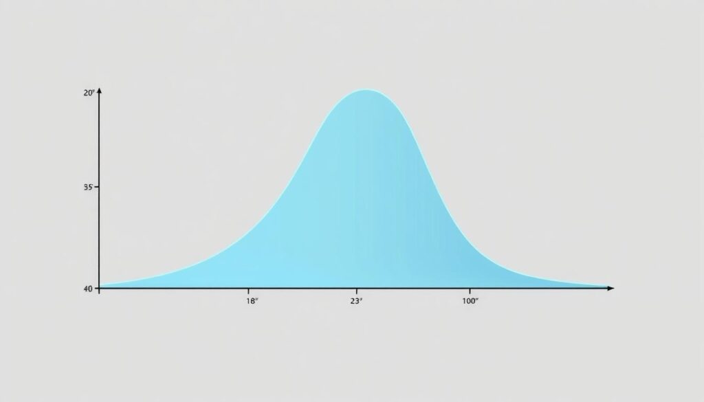
Why do methods like t-tests and regression demand this specific distribution? The bell curve’s symmetry allows accurate probability calculations. Standard deviations become meaningful markers. Mean values gain predictive power.
Consider pharmaceutical research. When testing drug efficacy, scientists assume reaction times follow this pattern. This assumption lets them calculate safe dosage ranges. Without it, confidence intervals lose reliability.
| Analytical Scenario | Normal Data | Non-Normal Data |
|---|---|---|
| Hypothesis Testing | Accurate p-values | False conclusions |
| Quality Control | Stable processes | Missed defects |
| Financial Forecasting | Precise risk models | Erratic predictions |
Implications for Models and Inferences
Violating the normality requirement doesn’t just skew numbers—it warps decision-making. A marketing team might misjudge campaign success. An engineer could overlook machinery wear patterns.
The Central Limit Theorem offers partial protection. With sufficient sample sizes, averages tend toward normality. But real-world data often needs adjustments. Square roots or log transformations frequently rescue skewed datasets.
Professionals face a critical choice: reshape the distribution or switch to non-parametric methods. Each option preserves analytical integrity differently. The right decision depends on data characteristics and business goals.
Assessing Your Data Distribution
Diagnostic evaluation separates reliable insights from statistical mirages. Professionals combine visual tools and quantitative checks to reveal hidden patterns in their datasets. This dual approach ensures decisions rest on both intuitive understanding and mathematical rigor.
Visual Methods: Histograms and QQ-Plots
Histograms act as distribution X-rays. These bar charts show where values cluster and how they spread. A quick glance reveals right-skewed sales figures or bimodal customer wait times.
QQ-plots take visualization deeper. By plotting sample quantiles against theoretical normal values, they highlight subtle deviations. Curved patterns suggest transformation needs, while straight lines confirm normality.
Statistical Tests for Normality
Numerical tests add precision to visual checks. The Shapiro-Wilk exam excels with smaller samples (under 50 observations), while Kolmogorov-Smirnov handles larger datasets. Both generate p-values indicating normally distributed likelihood.
| Method | Purpose | Strength | Limitation |
|---|---|---|---|
| Histogram | Shape visualization | Instant pattern recognition | Subjective interpretation |
| QQ-Plot | Deviation analysis | Identifies specific outliers | Requires statistical literacy |
| Shapiro-Wilk | Small sample testing | High sensitivity | Sample size restrictions |
| Kolmogorov-Smirnov | Large dataset analysis | Distribution flexibility | Lower power in small samples |
Combining these approaches creates safety nets. Visual tools explain why data behaves unusually, while statistical tests confirm whether deviations matter. Together, they guide transformation choices without over-relying on single metrics.
Techniques for Transforming Data for Normality
Choosing the right moment to adjust dataset patterns separates effective analysis from misleading results. Not every deviation demands intervention—seasoned analysts weigh statistical necessity against practical interpretation.
When and Why to Transform Your Data
Mild irregularities often pose minimal risk. Parametric tests can tolerate slight skewness, especially with large samples. But pronounced distributions resembling mountain slopes—not gentle hills—signal essential transformation needs.
Three scenarios demand action:
- Skewness exceeding ±1 for critical analyses
- Visible outliers distorting central tendencies
- Model assumptions repeatedly failing diagnostic checks
| Skew Type | Solution | Common Use Cases |
|---|---|---|
| Right-skewed | Logarithm | Income levels, website traffic |
| Left-skewed | Square root | Response times, inventory counts |
| Extreme values | Reciprocal | Rare event measurements |
Financial analysts frequently transform data using logarithms to stabilize stock volatility patterns. Biologists apply square roots to species counts for clearer ecological trends. These adjustments make data speak its truths more clearly.
Effective transformation balances mathematical rigor with stakeholder communication. While cubic roots might optimize models, simpler methods often win when explaining results to non-technical teams. The goal? Actionable insights—not just statistical elegance.
Addressing Outliers and Their Impact
Outliers lurk in datasets like uninvited guests—unexpected, disruptive, yet often revealing. These extreme values distort patterns and challenge assumptions about process stability. While their presence may signal non-normal distributions, smart analysts treat them as clues rather than nuisances.
Identifying Outliers in Data
Effective detection blends statistical tools with contextual awareness. Common methods include:
- Z-scores flagging values beyond ±3 standard deviations
- Interquartile range (IQR) analysis
- Visual inspections using box plots
Domain knowledge transforms numbers into narratives. A $10 million sales spike might seem anomalous—until you recall a one-time corporate merger. This fusion of math and meaning prevents misdiagnosis.
| Method | Strength | Weakness |
|---|---|---|
| Z-scores | Simple calculation | Sensitive to mean shifts |
| IQR | Robust to extremes | Ignores distribution shape |
| Box plots | Visual clarity | Subjective interpretation |
Strategies for Managing Outliers
Validation comes first. Check for data entry errors—a misplaced decimal can masquerade as an outlier. Genuine extremes demand deeper investigation:
- Determine recurrence likelihood
- Assess impact on business goals
- Choose accommodation or removal
Manufacturing teams might keep rare defect spikes if safety protocols demand worst-case planning. Conversely, marketers could exclude holiday sales surges when modeling regular campaigns. Strategic outlier management balances statistical purity with operational reality.
Advanced techniques like Winsorizing (capping extremes) or using robust regression maintain analytical power while minimizing distortion. The key lies in documenting decisions transparently—future analysts should understand why specific values received special treatment.
Box-Cox Transformation Explained
Modern analysts face a recurring challenge: finding the right mathematical lever to reshape stubborn datasets. The Box-Cox method solves this by unifying multiple adjustment strategies into one adaptable formula.
Concept and Formula
This technique uses a single parameter (λ) to create a spectrum of adjustments. The equation:
y = (x^λ – 1)/λ when λ ≠ 0
y = ln(x) when λ = 0
covers logarithmic, square root, and reciprocal operations. A λ of 0.5 straightens right-skewed measurements, while λ = -1 handles extreme left skews.
Determining the Optimal Lambda
Maximum Likelihood Estimation (MLE) statistically identifies the ideal λ. Analysts also test values between -5 and +5, comparing results through Q-Q plots or goodness-of-fit tests. Three factors guide selection:
- Statistical normality metrics
- Interpretability of transformed values
- Compatibility with analytical models
Financial teams might choose λ = 0 (log) for stock returns—even if λ = 0.2 offers slightly better normality—because logarithmic scales are industry-standard. This balance between precision and practicality defines successful implementation.
Johnson Transformation: A Robust Alternative
For stubborn datasets resisting simpler methods, a three-parameter approach unlocks hidden patterns. The Johnson system adapts to nearly any distribution shape through its SU, SB, and SL families. Unlike single-parameter solutions, this method combines flexibility with precision.
Mastering the Transformation Toolkit
The Johnson family offers distinct pathways:
- SU handles unbounded measurements with complex skewness
- SB manages values confined within specific ranges
- SL addresses lognormal-type patterns
Each method uses eta, epsilon, and lambda parameters to reshape distributions. This multi-variable optimization often achieves better normality than Box-Cox transformations.
Strategic Implementation Guidelines
Choose Johnson when:
- Critical analyses demand near-perfect normality
- Box-Cox fails to stabilize variance
- Multiple distribution quirks coexist
Financial modelers might select SU for volatile market metrics, while engineers could apply SB to bounded pressure readings. The optimal lambda emerges through iterative testing, balancing statistical rigor with practical interpretation.
While more complex, Johnson transformations become indispensable for high-stakes scenarios. They transform erratic datasets into reliable foundations for predictive models—without distorting underlying truths.
FAQ
Why does normality matter in statistical models?
Many parametric tests—like t-tests or linear regression—assume data follows a normal distribution. Violating this assumption can skew p-values, confidence intervals, and model accuracy. Transforming non-normal data ensures results are reliable and hypotheses are tested correctly.
How do I check if my data is normally distributed?
Start with visual tools like histograms or QQ-plots to spot deviations from the bell curve. Follow up with statistical tests like Shapiro-Wilk or Kolmogorov-Smirnov. These methods help quantify how closely your data aligns with a normal distribution.
What if transformations don’t make my data normal?
If transformations like Box-Cox or Johnson fail, consider non-parametric alternatives (e.g., Mann-Whitney U test). Outliers or skewed sample sizes might also distort results. Reassess data collection methods or use robust statistical techniques that don’t require normality.
When should I use the Johnson transformation over Box-Cox?
The Johnson system handles a wider range of distributions, including bimodal or heavily skewed data. Unlike Box-Cox—which requires positive values—Johnson transformations work with zero or negative values, offering flexibility for complex datasets.
Can outliers affect normality transformations?
Yes. Extreme values distort mean and variance, making transformations less effective. Use methods like the IQR rule or Mahalanobis distance to identify outliers first. Depending on their cause, you might winsorize, remove, or segment them before applying transformations.
Does transforming data change its meaning?
Transformations alter the scale—not the underlying relationships. For example, a log transform compresses large values but preserves rank order. Always interpret results in the transformed context or back-transform values for reporting.
How does the Box-Cox method determine the best lambda?
The Box-Cox algorithm uses maximum likelihood estimation to find the lambda (λ) that maximizes normality. Tools like Python’s SciPy or R’s MASS package automate this process, testing values between -5 and 5 to optimize the transformation.
Are there cases where normality isn’t necessary?
Yes. Non-parametric tests (e.g., Wilcoxon signed-rank) or large sample sizes (n > 30) often bypass normality assumptions due to the Central Limit Theorem. However, severely skewed data may still require transformations for accurate analysis.


