Did you know 68% of all data points naturally cluster within one unit of spread from the average in most datasets? This invisible boundary—often overlooked—holds the key to understanding predictability in everything from stock markets to weather forecasts.
In statistics, two concepts act as compasses for navigating numerical chaos. The first quantifies squared deviations from the mean, while the second translates this value into intuitive units. Together, they transform raw numbers into a clear story about consistency, risk, and reliability.
Professionals rely on these tools to distinguish noise from trends. Financial analysts use them to assess investment volatility. Quality control teams apply them to maintain production standards. Researchers leverage them to validate experiments—all through a lens grounded in mathematics.
Mastering these measures unlocks sharper decision-making. They reveal whether a sales spike reflects genuine growth or random fluctuation. They help educators identify outlier student performance. Most importantly, they turn abstract digits into strategic insights.
Key Takeaways
- Core statistical tools quantify how data spreads around an average value
- One metric derives from the square root of another, enhancing real-world interpretation
- 68% of values typically fall within a specific range from the mean
- Critical for assessing risks in finance and quality in manufacturing
- Converts numerical complexity into actionable business intelligence
- Builds foundation for advanced analytics and machine learning models
Understanding the Basics of Variance and Standard Deviation
What separates meaningful patterns from random noise in datasets? The answer lies in two statistical workhorses that measure how numbers spread out. These tools don’t just crunch digits—they reveal whether changes matter.
Defining Variance in Statistics
Variance acts as a mathematical magnifying glass. It calculates the average of squared differences between each value and the arithmetic mean. By squaring deviations, it eliminates negative signs that could distort the true spread. This process creates σ²—a value representing how tightly or loosely numbers cluster.
Consider test scores: If most students score near 75%, variance remains low. Wide-ranging results create higher values. This metric becomes the foundation for assessing consistency in manufacturing, finance, and scientific research.
Explaining Standard Deviation and Its Importance
While variance quantifies spread mathematically, standard deviation translates it into practical terms. By taking the square root of σ², analysts regain the original data’s units. A measurement consistency emerges—dollars stay dollars, inches remain inches.
This unit alignment enables direct comparisons. Investors gauge stock volatility in percentage terms. Quality managers assess product dimensions against tolerance ranges. Unlike variance’s abstract squared units, standard deviation speaks the language of the original dataset, making insights immediately actionable.
Variance and Standard Deviation: Key Concepts and Terminology
How do statisticians separate reliable patterns from random chance? The answer lies in mastering foundational relationships and recognizing critical distinctions between complete datasets and partial snapshots.
Relationship Between Mean, Variance, and Deviation
The arithmetic mean acts as ground zero for variability measurements. Every deviation gets calculated from this central anchor point—a process that transforms abstract differences into quantifiable values.
Squared deviations eliminate negative distances, creating a unified measure of spread. This squared value becomes variance, which then gets converted back to original units through its square root. The result? A practical gauge of dispersion that speaks the dataset’s native language.
Differences Between Population and Sample Data
Complete datasets (populations) use straightforward calculations: divide by total observations (N). Partial datasets (samples) require adjusted math—dividing by N-1. This degrees of freedom correction accounts for missing information in subset analyses.
Consider market research: Surveying every customer yields population metrics. Polling 1,000 shoppers produces sample statistics needing N-1 adjustments. The choice impacts accuracy—population formulas assume full visibility, while sample methods acknowledge inherent uncertainty.
Professionals who grasp this distinction avoid critical errors. They select formulas based on data scope, ensuring analyses reflect true variability rather than methodological artifacts.
Deep Dive into Variance and Standard Deviation Formulas
How do analysts transform raw numbers into reliable insights? The answer lies in precise mathematical frameworks that quantify spread with surgical accuracy. These equations form the backbone of statistical analysis, bridging theoretical concepts and real-world applications.

Population Variance and Standard Deviation Formulas
Complete datasets demand specific calculations. The population variance formula (σ² = Σ(Xi-μ)²/N) averages squared deviations from the mean. Here, μ represents the true average, while N counts every existing data point.
Taking the square root of this result produces population standard deviation (σ). This step converts abstract squared units back to their original measurement scale. Manufacturing teams use these formulas when assessing full production batches—no estimations required.
Sample Variance and Standard Deviation Formulas
Partial datasets introduce uncertainty. The sample variance formula adjusts for missing information by dividing squared deviations by n-1 instead of n. This degrees of freedom correction prevents underestimation when working with limited observations.
Market researchers apply sample standard deviation (s = √[Σ(xi-x̄)²/(n-1)]) to survey data. The x̄ symbol denotes sample mean—a temporary anchor point until more data emerges. This approach acknowledges the inherent variability in working with subsets.
Applying the Concepts: Real-World Examples and Calculations
Numbers gain true meaning when applied to real-world scenarios. Let’s explore how professionals calculate spread metrics using tangible examples—from canine physiology to gaming probability.
Step-by-Step Calculation of Variance
Consider five dogs with heights of 600mm, 470mm, 170mm, 430mm, and 300mm. The mean height equals 394mm. Here’s how to find variance:
- Subtract each value from the mean: 206, 76, -224, 36, -94
- Square these differences: 42,436; 5,776; 50,176; 1,296; 8,836
- Sum the squares: 108,520
- Divide by total observations: 108,520 ÷ 5 = 21,704
This average squared difference becomes our variance. For dice rolls, similar calculations yield 2.917 variance when analyzing outcomes from 1 to 6.
Computing Standard Deviation in Everyday Contexts
To convert variance into practical terms, take its square root. The dog height example produces 147mm (√21,704). This value shows typical deviations from the average—crucial for assessing consistency in manufacturing or animal growth patterns.
When working with samples, adjust calculations by dividing squared differences by n-1 instead of n. The same dog measurements analyzed as a sample yield 27,130 variance and 165mm spread. This distinction prevents underestimation in market research or quality control studies.
Dice probability demonstrates versatility—1.708 units of spread reveal how outcomes cluster around the mean. Such calculations empower professionals to quantify uncertainty in finance, gaming, and scientific experiments.
Practical Implications of Variance and Standard Deviation
In the realm of data analysis, numbers tell stories of consistency and risk. Professionals rely on two interconnected metrics to separate predictable patterns from chaotic fluctuations. These tools don’t just measure spread—they inform strategy.
Interpreting Variability in Data Sets
Low dispersion values near zero signal tight clustering around averages. Think factory parts matching exact specifications or repeated lab experiments with minimal error. High values? They’re red flags—like erratic stock prices or inconsistent customer wait times.
Approximately 68% of observations naturally fall within one unit of spread from the mean in normal distributions. This empirical rule helps analysts quickly assess outlier likelihood. For example, quality managers might investigate measurements beyond this range as potential defects.
Using Standard Deviation for Statistical Analysis
Financial experts prefer standard deviation for volatility checks because it speaks their language. A stock’s 5% monthly spread means more than abstract squared percentages. It directly compares to historical averages and competitor performance.
Variance, while less intuitive, powers portfolio optimization. Squared deviations reveal how assets interact risk-wise—a critical insight when balancing high-risk and stable investments. Together, these metrics form a decision-making framework applicable across industries.
Consider these applications:
- Low spread values guide process standardization efforts
- High variability prompts root-cause investigations
- Unit consistency enables cross-department communication
Conclusion
Mathematics gains predictive power through tools that quantify uncertainty. These paired metrics—one rooted in squared differences, the other in practical units—turn raw numbers into decision-making fuel. Their calculations reveal hidden patterns across fields, from drug trials to supply chain management.
The choice between population and sample formulas matters. Complete datasets use exact averages, while partial observations require adjusted math. This distinction prevents skewed conclusions when analyzing market trends or manufacturing outputs.
Why square deviations instead of using absolute values? Squaring eliminates canceling effects between positive and negative differences while emphasizing extreme variations. The result: a truer reflection of spread that powers risk assessment models and quality control systems.
Professionals wield these concepts to separate signal from noise. Low values indicate consistency in product dimensions or stock performance. High values flag potential outliers in clinical research or customer behavior. Every dataset tells a story—these metrics provide the vocabulary to interpret it accurately.
FAQ
Why do we square differences when calculating variance?
Squaring differences emphasizes larger deviations from the mean, ensuring positive values and simplifying mathematical properties like differentiability. It also penalizes outliers more heavily, providing a clearer picture of data spread.
How does sample data differ from population data in calculations?
Sample formulas use n−1 (Bessel’s correction) instead of N to account for estimation bias. This adjustment improves accuracy when generalizing results from a subset to an entire group.
What does a high standard deviation indicate about a dataset?
A higher value suggests greater dispersion, meaning data points are farther from the mean. For example, test scores with a standard deviation of 15 show more variability than those with 5.
When should I use variance instead of standard deviation?
Variance is useful in statistical tests like ANOVA, where squared units are manageable. Standard deviation is preferred for direct interpretation, as it shares the original data’s units (e.g., meters, dollars).
Can these metrics be applied to non-numerical data?
No—they require quantitative measurements. For categorical data, use metrics like mode or frequency analysis to assess patterns.
How do outliers impact these measures?
Extreme values disproportionately increase both variance and standard deviation. Analysts often use tools like interquartile range (IQR) for skewed datasets to reduce outlier influence.
What’s a practical example of using these concepts?
Investors use standard deviation to assess portfolio risk. A fund with a higher value might offer larger returns but carries more volatility compared to a stable, low-deviation option.